

Ⅰ. Introduction
Ⅱ. Institutional Background, Prior Research and Hypotheses
1. The October 2021 Tariff Reform
2. Prior Research and the Differentiation of This Study
3. Hypotheses
Ⅲ. Data and Research Design
1. Data Sources
2. Sample and Exposure Measures
3. Specification
4. Descriptive Statistics
Ⅳ. Results
1. Baseline
2. Dynamics
3. Where the Level Shock Goes
4. Cross-sectional Variation
5. Sensitivity
6. Comparison with the Industry-List Design
Ⅴ. Conclusion
Ⅰ. Introduction
Electricity marketisation changes both the level and the variability of electricity prices, and these two dimensions may affect firms through different channels. A higher expected electricity price compresses margins when pass-through is incomplete and encourages substitution away from electricity-intensive production. Greater price variability instead increases uncertainty about future operating costs and cash flows, which may affect investment and the required return on equity when external financing is costly (Froot et al., 1993; Minton and Schrand, 1999). Related evidence shows that uncertainty postpones irreversible investment (Bloom et al., 2007; Bloom, 2009) and that investors respond to the smoothness of realised corporate performance (Rountree et al., 2008). This distinction suggests that the first and second moments of an input price should not necessarily be treated as the same economic exposure.
China’s October 2021 electricity pricing reform provides a setting in which the two dimensions can be examined jointly. The reform widened the trading band around provincial coal-fired power benchmark tariffs, abolished industrial and commercial catalogue tariffs, and removed the upward cap for energy-intensive users. From 2022, industrial and commercial firms became more directly exposed to market-referenced electricity prices. The reform affected provincial markets unevenly. Provinces with higher average market premia were not generally those with greater month-to-month price variability, and the cross-sectional correlation between the two provincial moments is only 0.104. Liberalisation in other electricity markets has similarly altered both price levels and price variability (Borenstein, 2002; Joskow, 2008). The Chinese setting is particularly useful because these two changes display substantial geographic separation.
Existing research has primarily examined the level of energy prices. Energy costs affect productivity, input substitution, technological change, and production location (Popp, 2002; Linn, 2008; Aghion et al., 2016; Abeberese, 2017; Ganapati et al., 2020; Marin and Vona, 2021; Saussay and Sato, 2024), while firms pass a substantial share of cost increases through to output prices (Fabra and Reguant, 2014). Studies of administered electricity pricing in China generally identify treatment using administratively designated industries or policy coverage (Zheng et al., 2021; Qu et al., 2022; Yi et al., 2024; Xie and Huang, 2025; Zhao and Zhang, 2025). Adjacent research examines electricity shortages and rationing rather than price risk (Fisher-Vanden et al., 2015; Allcott et al., 2016). These studies establish important real effects of energy-market interventions, but they do not generally separate changes in the expected price from changes in its variability.
The distinction is also relevant to the literature on priced uncertainty. Political and regulatory uncertainty is associated with investment and risk premia (Julio and Yook, 2012; Pástor and Veronesi, 2013; Baker et al., 2016; Gulen and Ion, 2016; Kelly et al., 2016), while environmental and transition exposures are reflected in financial markets when their future consequences are uncertain (Engle et al., 2020; Krueger et al., 2020; Bolton and Kacperczyk, 2021; Ilhan et al., 2021; Pástor et al., 2021; Bolton and Kacperczyk, 2023; Hsu et al., 2023; Sautner et al., 2023). Electricity price variability represents a related operating risk, but one that arises from a dated institutional reform and can be measured using provincial price information.
We construct two continuous firm-level exposure measures from the same pre-reform firm characteristic. Pre-reform electricity and fuel cost intensity is combined separately with the mean provincial market premium and the monthly volatility of that premium. The resulting level and risk exposures are entered jointly in a continuous-exposure difference-in-differences specification. The sample contains 25,925 firm-year observations for 3,412 non-financial Chinese A-share firms from 2017 to 2024. Firm fixed effects absorb time-invariant exposure differences, while the preferred specification further includes industry-by-year and province-by-year fixed effects. Standard errors are clustered by province, where the electricity price regime varies.
The results indicate that exposure to price variability has the more robust association with the implied cost of equity. In the preferred specification, a one-standard-deviation increase in risk exposure is associated with a 0.313 percentage point higher implied cost of equity. The coefficient remains positive across alternative fixed-effect structures, when provincial exposure is reconstructed using only 2022 price information, when exposure is rebuilt year by year from information available up to each fiscal year, and when the spot-market pilot designation announced before the reform replaces realised volatility as the source of cross-provincial variation. The dynamic estimates are close to zero before the reform and become positive from 2022 onward. In contrast, level exposure is statistically indistinguishable from zero in this design once the lower-order energy-intensity interaction is included.
The two exposures also appear in different firm outcomes. Level exposure is associated with lower gross margins, lower energy intensity, and greater energy-saving innovation, consistent with the operating responses documented in the energy-price literature. Risk exposure is associated with higher realised cash-flow volatility and lower capital expenditure. Adding realised cash-flow volatility to the cost-of-equity specification attenuates the risk coefficient, which is consistent with cash-flow volatility representing one possible channel, although the comparison does not identify mediation and the paper does not assign a share of the association to it. The association is also weaker among firms disclosing long-term bilateral power purchase agreements, which is consistent with, but does not by itself establish, the risk-management role of contractual hedging documented in prior research (Smith and Stulz, 1985; Allayannis and Weston, 2001; Bartram et al., 2011; Campello et al., 2011; Pérez-González and Yun, 2013; Gilje and Taillard, 2017).
This study contributes by separating the level and variability of the same input price and by measuring exposure continuously rather than solely through an administrative industry classification. A conventional energy-intensive industry design produces a sizeable post-reform difference when used alone, but that coefficient becomes close to zero when the continuous exposures are introduced jointly, while the risk coefficient remains stable. Substantial exposure variation also remains within industries. This distinction is consistent with the broader difference- in-differences literature showing that binary and exposure-weighted treatment designs can recover different objects when treatment intensity varies within groups (de Chaisemartin and D’Haultfœuille, 2020; Callaway and Sant’Anna, 2021; Goodman-Bacon, 2021; Sun and Abraham, 2021; Borusyak et al., 2022; Callaway et al., forthcoming). Because exposure is continuous, the coefficients are read throughout as differences in post-reform changes between firms with different exposure intensities, and Section Ⅲ.3 states the assumptions under which that comparison carries a causal interpretation.
The evidence therefore suggests that evaluations of electricity marketisation should distinguish changes in average prices from changes in price variability. In this setting, the former is more closely associated with operating adjustment, whereas the latter has the more consistent association with the implied cost of equity. Section Ⅱ presents the institutional background, prior research, and hypotheses. Section Ⅲ describes the data and empirical design. Section Ⅳ reports the results, and Section Ⅴ concludes.
Ⅱ. Institutional Background, Prior Research and Hypotheses
1. The October 2021 Tariff Reform
China’s coal-power tariff had been anchored since 2004 to a provincial benchmark set administratively. From 2019 the benchmark could move within a band of minus fifteen to plus ten per cent, but in practice the upward half of the band was seldom used, and industrial and commercial users continued to face a catalogue tariff. Through 2021 a combination of high coal input costs and administered output prices compressed generator margins to the point of widespread output curtailment. Liberalisation experience elsewhere suggests that the transition from an administered to a market price changes the statistical properties of the price and not only its average level (Borenstein, 2002; Joskow, 2008).
The 12 October 2021 notice changed three parameters simultaneously. The permitted band became symmetric at plus or minus twenty per cent. The industrial and commercial catalogue tariff was abolished, so that users either transact in the market or are served by a grid company at a market-referenced price. And users classified as energy-intensive were exempted from the upward twenty per cent limit, so that their transaction prices could rise without an administrative ceiling. The market share of traded electricity, which had been below seventeen per cent of generation in 2016, reached 61.4 per cent of national consumption by 2023, of which medium- and long-term bilateral contracts accounted for approximately seventy-eight per cent.
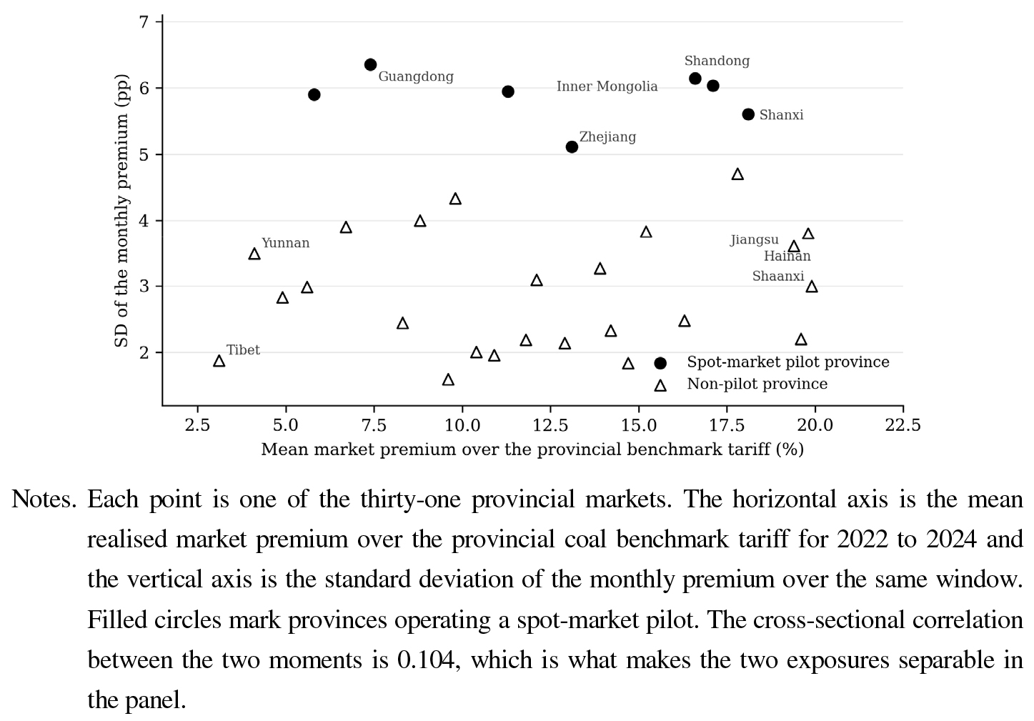
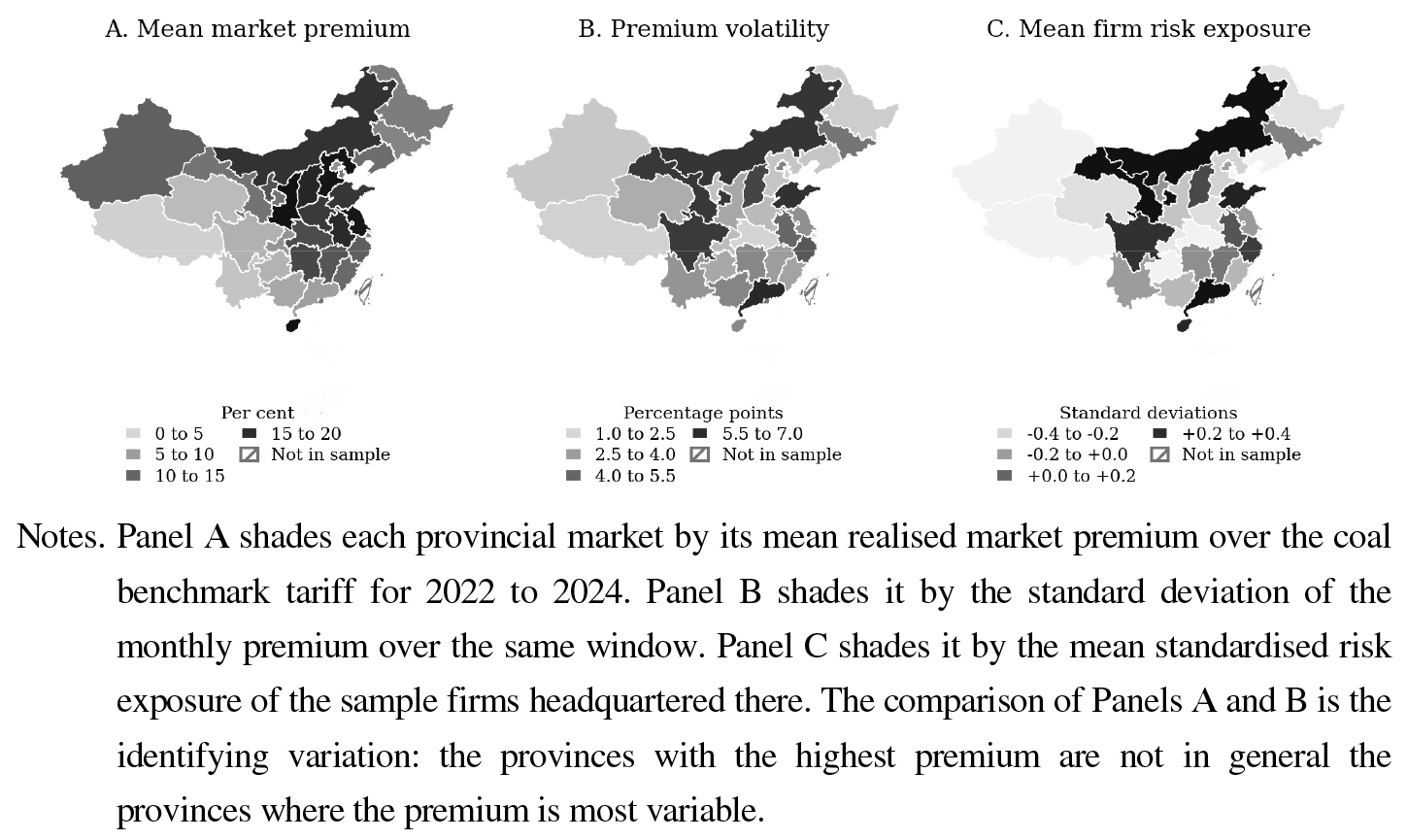
Two features of the resulting price process matter for this paper. The first is that realised premia over the benchmark differ substantially across provinces. Reported 2022 annual-contract outcomes include a premium of 19.36 per cent in Jiangsu, where the average tariff of 466.78 yuan per megawatt hour sat just below the 469.2 ceiling, and 7.35 per cent in Guangdong, which had traded at a discount of 11.56 per cent in the preceding year. The second is that the provinces where the price is most variable within the year are the spot-market pilot provinces, and these are a different set from the provinces with the highest annual premium. [Figure 1] shows the resulting near-orthogonality between the mean premium and its monthly standard deviation across the thirty-one provincial markets, and [Figure 2] maps the two moments alongside the firm-level risk exposure they generate.
What market participants could observe before 2022 differs across the two moments, and the distinction matters for how the exposures are read. The direction of the level change was known from the notice itself, and the annual-contract results for 2022 that provincial trading centres published in December 2021 already placed several large provinces, Jiangsu among them, at or near the twenty per cent ceiling, so the ordering of provinces by expected premium was partly visible before any 2022 price was realised. The magnitude of realised premia, and above all the month-to-month variability of the premium, were not observable in advance; they are outcomes of the first three years of trading. What was known in advance about variability was institutional. The first eight spot-market pilot regions, Guangdong, western Inner Mongolia, Zhejiang, Shanxi, Shandong, Fujian, Sichuan and Gansu, were designated in August 2017, and a second group of six, Shanghai, Jiangsu, Anhui, Liaoning, Henan and Hubei, was announced in April 2021, so every pilot designation used in this paper predates the 12 October 2021 notice. A firm in a pilot province could anticipate that its provincial price would be settled at a higher frequency and would therefore be more variable, without knowing by how much. The premium and volatility measures used in the baseline are accordingly realised, post-reform descriptions of the price regime each province entered rather than forecasts investors held in 2022. Section Ⅲ.2 explains how that construction is handled, and Section Ⅳ.5 reports specifications that replace the realised moments with information available at the time, including the pre-announced pilot designation.
2. Prior Research and the Differentiation of This Study
Four strands of prior work bear on the question, and this study differs from each along an identifiable dimension rather than by incremental sample extension.
The first strand studies administered energy price instruments in China. The differential electricity pricing programme surcharges firms in restricted and eliminated categories within eight designated energy-intensive industries, and the associated work finds productivity and fuel-consumption responses (Zheng et al., 2021; Qu et al., 2022). The treatment there is a binary industry-list indicator applied uniformly across provinces. The present setting supplies continuous, province-specific variation that is measured rather than assigned, which permits identification within industry-by-year cells and therefore survives the inclusion of industry-by-year fixed effects. The industry-list design cannot do this, because its treatment indicator is collinear with industry. The programme has been evaluated for productivity and fuel-consumption responses (Zheng et al., 2021; Qu et al., 2022), and the more recent Chinese evidence on trading pilots and price distortions is organised the same way, around who is covered rather than around how exposed each firm is (Yi et al., 2024; Xie and Huang, 2025; Zhao and Zhang, 2025).
The second strand studies electricity supply rather than price: shortages, rationing and outages, and their consequences for productivity and self-generation (Fisher-Vanden et al., 2015; Allcott et al., 2016; Abeberese, 2017). Quantity rationing and price marketisation are different instruments with different hedging technologies available against them, and the reform we study is explicitly the substitution of the second for the first.
The third strand studies energy and carbon price shocks in developed markets, where the identifying variation is typically a cross-country or cross-establishment difference in energy price levels (Ganapati et al., 2020; Marin and Vona, 2021; Saussay and Sato, 2024). This work is concerned with pass-through, employment and location, and treats the price level as the treatment. The volatility of that price is generally not separated out, in part because in liberalised markets firms have had hedging instruments available for long enough that the second moment is not a new object. That work also establishes that firms pass a substantial share of an energy cost increase through to prices rather than absorbing it (Fabra and Reguant, 2014; Ganapati et al., 2020), and that the response to a higher price is partly a change in the direction of innovation (Popp, 2002; Linn, 2008; Aghion et al., 2016).
The fourth strand studies the equity pricing of environmental and climate risk, and establishes that investors require compensation for exposures that are prospective and imprecisely measured (Krueger et al., 2020; Bolton and Kacperczyk, 2021; Ilhan et al., 2021; Sautner et al., 2023). The exposure in that literature is an emissions or transition risk. Here it is an input price whose second moment changed on a dated administrative decision, which supplies a sharper timing than transition-risk settings generally allow. The measured exposures in that work are emissions- or transition-based (Engle et al., 2020; Krueger et al., 2020; Bolton and Kacperczyk, 2021; Ilhan et al., 2021; Pástor et al., 2021; Bolton and Kacperczyk, 2023; Hsu et al., 2023; Sautner et al., 2023). Here the exposure is a price process, its date is known, and its cross-sectional variation is administrative rather than behavioural.
The differentiation of this study can therefore be stated in one sentence. Prior work asks how much a firm pays for energy and what it does in response; this paper asks how uncertain that payment became and how the required return on equity varied with that uncertainty, holding the payment constant.
3. Hypotheses
A shock to the level of a variable input price is, in a standard framework, a shock to the conditional mean of future cash flows. If it is anticipated and passed through only in part it compresses margins and induces substitution away from the input, and it need not change the rate at which those cash flows are discounted. A shock to the variability of the same price acts on the conditional variance instead. Where investors are imperfectly diversified against it, or where a wider distribution of cash flows raises the probability of distress or of foregone investment, the required return rises. This asymmetry is not a modelling convenience. It follows from the frictions that make cash-flow volatility costly in the first place (Smith and Stulz, 1985; Froot et al., 1993; Minton and Schrand, 1999; Bloom et al., 2007), and from the evidence that policy-induced uncertainty carries a premium (Julio and Yook, 2012; Pástor and Veronesi, 2013; Baker et al., 2016; Gulen and Ion, 2016; Kelly et al., 2016). Each of the four hypotheses below isolates one implication of it.
Marketisation replaced a price the firm could predict with one it cannot. For a producer whose technology requires electricity in close to fixed proportions over the short run, the width of the distribution of next year’s electricity bill passes into the width of the distribution of operating cash flow, and it does so in proportion to how electricity-dependent the firm is and how variable the price in its provincial market has become. If investors price this the way they price other second-moment exposures they cannot diversify away, the compensation should be visible in the discount rate applied to the firm after the reform and absent from it before.
H1. Post-reform, risk exposure is positively associated with the implied cost of equity.
The level of the price reaches the firm through a different margin. A producer facing a permanently higher tariff earns a lower expected operating margin unless it can pass the increase on, and it has an incentive to substitute towards less electricity-intensive production and towards technologies that consume less of it, which is the response documented for energy prices in other settings (Popp, 2002; Linn, 2008; Aghion et al., 2016; Ganapati et al., 2020; Marin and Vona, 2021). None of that requires the discount rate to move. If the two properties of the price are genuinely distinct objects, the level exposure should be legible in operating outcomes while adding little to the cost of equity once the risk exposure is held constant.
H2. Post-reform, level exposure is associated with gross margins, energy intensity and energy-saving innovation, but adds little to the implied cost of equity once risk exposure is held constant.
If what H1 describes is compensation for the exposure of cash flows, and not for something merely correlated with that exposure, the association should have an observable intermediate step. A firm more exposed to a variable electricity price should report more volatile realised operating cash flow, and the coefficient on risk exposure in the cost-of-equity specification should be smaller once that realised volatility is controlled for. The test is a weak one. Realised volatility is itself an outcome, and conditioning on it cannot separate a mediated effect from a common cause, so H3 is stated as a prediction about the behaviour of a coefficient rather than as a mediation claim. A channel that left no trace in realised cash flows would nonetheless be difficult to sustain, which is what makes the exercise worth running.
H3. The association in H1 is accompanied by higher realised cash-flow volatility, and the coefficient on risk exposure is attenuated after controlling for realised cash-flow volatility.
Firms are not passive with respect to an exposure of this kind. A long-term bilateral power purchase agreement fixes the price over a contracted volume and removes the corresponding part of the price process from the firm’s cash flows, which is the mechanism through which hedging has been found to lower risk and, in several settings, to raise firm value (Smith and Stulz, 1985; Allayannis and Weston, 2001; Bartram et al., 2011; Campello et al., 2011; Pérez-González and Yun, 2013; Gilje and Taillard, 2017). If the association in H1 is compensation for bearing the marketised price, it should be weaker among firms that disclose having contracted it away, and it should not be weakened by firm characteristics that leave the exposure in place. Because contract disclosure records presence rather than contracted volume and is itself a choice, H4 is a prediction about an observed difference between disclosing and non-disclosing firms.
H4. The association in H1 is weaker for firms with contractual hedges against the marketised price, namely disclosed long-term bilateral power purchase agreements.
Ⅲ. Data and Research Design
1. Data Sources
Firm-level accounting and market data are drawn from the CSMAR database and cross-checked against WIND. Institutional parameters, namely the reform date, the band width, the catalogue-tariff abolition and the energy-intensive exemption, are taken from the 12 October 2021 notice. Provincial price data, namely the mean and monthly standard deviation of the market premium over the benchmark tariff, are compiled from the annual and monthly settlement bulletins of the thirty-one provincial power trading centres for 2022 to 2024, and the 2022 annual-contract outcomes for Jiangsu, Guangdong and the provinces trading near the ceiling are cross-checked against the figures reported in the trade press. Appendix Table A1 lists, for each of the thirty-one provincial markets, the mean premium, its monthly standard deviation, the number of monthly settlement observations underlying each and the spot-pilot designation and its date. Spot-market pilot status follows the pilot designations of the National Development and Reform Commission and the National Energy Administration. Analyst forecasts used to construct the implied cost of equity come from the CSMAR analyst forecast file, and disclosures of long-term bilateral power purchase contracts and of self-generation capacity are hand-collected from annual reports. Government subsidies received are taken from the CSMAR government-subsidy file, which records the fiscal transfers disclosed in the notes to the financial statements. For the 1,024 firms whose notes separate purchased electricity from fuel, the electricity item alone is used to construct the electricity-only intensity measure of Section Ⅳ.5.
2. Sample and Exposure Measures
The panel covers 3,412 non-financial A-share firms across thirty-one provincial markets and twenty-two industry groups over the fiscal years 2017 to 2024, giving 25,925 firm-year observations after attrition for listing timing, special treatment status and missing analyst coverage. The sample is assembled by taking A-share firms listed on the Shanghai and Shenzhen exchanges over the window and then excluding, in order, financial firms, firm-years under special treatment status, firm-years for which the disclosed electricity and fuel cost item is unavailable, and firm-years without the analyst coverage needed to construct the implied cost of equity. No interpolation, imputation or industry-mean substitution is applied to either the cost item or the forecast data; a firm-year that fails a screen is dropped. The resulting panel is unbalanced, and firms enter and leave it with listing timing and forecast coverage. The reform is dated to 2022, the first full pricing year after the October 2021 notice.
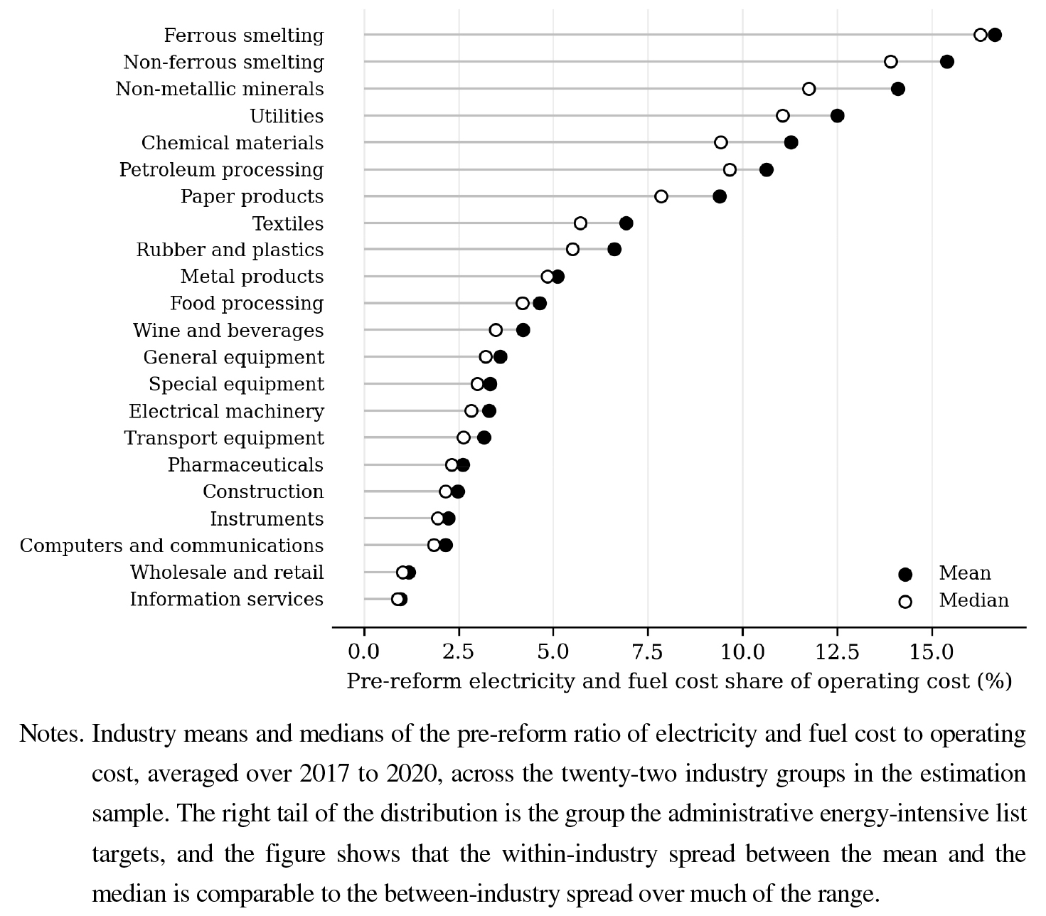
Pre-reform energy-cost intensity, denoted EI, is defined as the average ratio of disclosed electricity and fuel costs to operating costs over 2017 to 2020. Because the disclosed cost item combines purchased electricity and fuel, EI should be interpreted as an energy-cost intensity measure rather than as a pure measure of electricity dependence. Among the 1,024 firms that separately disclose purchased electricity and fuel costs, electricity accounts for 72.6 per cent of the combined item on average, and the cross-sectional correlation between the electricity-only and combined intensity measures is 0.91. Fuel-intensive firms are also not outside the reform: the energy-intensive classification that governs tariff treatment is defined on total energy use, and thermal-coal and market electricity prices co-move through the coal price. To the extent that the fuel component contains variation unrelated to the provincial electricity-price process, it introduces measurement error that would tend to attenuate the estimated exposure coefficient. Because fuel prices may also co-move with electricity prices, we do not interpret the combined measure as a purely classical measurement-error case. We therefore re-estimate the baseline using the electricity-only measure for the disclosing subsample in Section Ⅳ.5, where the measurement-error exercise is also reported. Its sample mean is 0.053 and its standard deviation is 0.058, with the ferrous and non-ferrous smelting, non-metallic mineral and utilities groups at the top of the distribution, as [Figure 3] shows. The provincial premium, Prem, is the mean realised market price premium over the provincial coal benchmark during 2022 to 2024, with a sample mean of 0.127. The provincial premium volatility, Vol, is the standard deviation of the monthly realised premium in the same window, with a sample mean of 0.041. The cross-sectional correlation between Prem and Vol across the thirty-one provinces is 0.104. Both provincial moments are computed from prices realised after the reform, so the exposure assigned to a firm describes the price regime the reform placed it in rather than a forecast an investor could have held in 2022. Section Ⅴ returns to what that construction implies for reading the dynamic profile. Column 5 of <Table 5> shows that the cost-of-equity association survives when both exposures are rebuilt from 2022 price information alone, and Section Ⅳ.5 reports two further constructions that use no information beyond what was available in each year: exposures rebuilt year by year from the settlement months observed up to and including that fiscal year, and a specification in which the pre-announced spot-pilot designation replaces realised volatility altogether.
The two exposures follow directly:
each standardised to zero mean and unit variance across firms, as in Eq. (1). Their correlation in the estimation panel is 0.747 and the variance inflation factor on the pair is 2.275. Section Ⅳ.5 reports specifications in which each exposure is orthogonalised against the other. The correlation arises because the two exposures share the firm characteristic EI and differ only in the provincial moment that scales it. When both enter jointly with the lower-order EI × Post term, the coefficient on RiskExp × Post is identified from the covariance between EI and the cross- provincial variation in Vol, holding the covariance between EI and Prem fixed, and symmetrically for LevelExp × Post. Because Prem and Vol are nearly uncorrelated across provinces, the two products are separable in the panel despite their 0.747 correlation, which is the common EI factor. The lower-order term absorbs any post-reform change common to energy-intensive firms in every province, and the province-by-year effects absorb any change common to every firm in a province, so each interaction coefficient is identified from the joint variation in energy intensity and one provincial moment, conditional on the other.
<Table 1>
Variable definitions
3. Specification
The baseline is a continuous-exposure difference-in-differences specification estimated by ordinary least squares:
where Eq. (2) is the estimating equation, ICC is the implied cost of equity in percentage points, computed as the average of a price-earnings-growth estimate and a residual-income estimate; Post equals one from 2022; a(i) and b(t) are firm and year fixed effects; and X is the control vector defined in <Table 1>. The term EI × Post is the lower-order interaction implied by the construction of the two exposures; column 1 of <Table 5> omits it and every later specification includes it. Firm fixed effects absorb both exposures in levels, so the two interaction coefficients are identified from the change in the exposure-outcome relation at the reform. Standard errors are clustered by province throughout, the level at which the price regime varies, and Section Ⅳ.5 reports alternatives. Extensions replace the year effects with industry-by-year effects, and then add province-by-year effects, so that they are identified from firms in the same industry and the same province in the same year that differ in pre-reform energy intensity. The implied cost of equity is estimated following the standard implementations of the residual-income and abnormal-earnings-growth approaches (Claus and Thomas, 2001; Gebhardt et al., 2001; Easton, 2004; Ohlson and Juettner-Nauroth, 2005), which are the measures whose relative performance has been assessed most closely in the literature (Botosan and Plumlee, 2005; Hail and Leuz, 2006; Hou et al., 2012), and whose measurement error is known to load on earnings and forecast properties (Francis et al., 2004). Appendix B sets out the two implementations used for ICC, the forecast horizon, the terminal growth assumption and the treatment of missing and negative forecasts.
Because exposure is continuous, β1 and β2 are not the effect of moving a firm from zero to positive exposure, and the object they recover needs to be stated. Callaway, Goodman-Bacon and Sant’Anna (forthcoming) show that a two-way fixed effects regression with a continuous treatment recovers a weighted average of comparisons between units with different treatment intensities, with weights that depend on the distribution of the treatment rather than on any economic quantity. Under the standard parallel trends assumption, that firms’ cost of equity would have evolved in parallel after 2021 regardless of exposure, those comparisons identify how the post-reform change in the cost of equity differs between more and less exposed firms among the firms that were in fact exposed. Reading the slope as the causal effect of a marginal increase in exposure requires a stronger assumption, which Callaway, Goodman-Bacon and Sant’Anna (forthcoming) call strong parallel trends: that the change a firm would experience at a given exposure level does not depend on the exposure level it actually received. The event-study estimates in Section Ⅳ.2 examine the first assumption in the pre-reform window. They do not examine the second, which concerns counterfactual responses at exposure levels a firm did not receive and is not testable from pre-reform data.
The paper therefore reads β1 as the post-reform difference in the implied cost of equity between firms one standard deviation apart in risk exposure, and not as the effect of a unit increase in exposure. Two features of the setting make the stronger assumption less demanding than it is in many applications. Exposure is the product of a technological characteristic fixed before the reform and a provincial price moment that firms did not choose, so the mechanism by which firms with different exposure levels would respond differently to the same level is not obvious, and Panel B of <Table 4> shows that firms at different exposure levels were similar on observed financial characteristics before the reform. Because the two-way fixed effects weights nonetheless place more weight on some parts of the exposure distribution than others, Section Ⅳ.5 also reports a binned specification in which exposure enters as quintile indicators interacted with Post, so that the shape of the response across the exposure distribution is visible without a linearity assumption.
4. Descriptive Statistics
<Table 2> reports the distribution of the estimation variables and <Table 3> the pairwise correlations among the principal ones. The mean implied cost of equity is 9.34 per cent with a standard deviation of 2.64 percentage points, which is within the range reported for Chinese listed firms. Gross margin averages 26.2 per cent, cash-flow volatility 4.37 per cent of assets, and capital expenditure 5.20 per cent of lagged assets. Neither exposure is meaningfully correlated with size, leverage, profitability, market-to-book or beta, with all such correlations below 0.01 in absolute value, which is consistent with the exposures being constructed from a technological characteristic and a location rather than from a financial one.
<Table 2>
Descriptive statistics
<Table 3>
Pairwise correlations
<Table 4> presents the design in its two-by-two form. Assigning the top tercile of risk exposure to treatment and the bottom tercile to control, and splitting at the reform, Panel A reports the four group-period means for each outcome with no controls and no fixed effects. The treated implied cost of equity moves from 9.014 to 10.228 per cent while the control moves from 9.069 to 9.500, a raw difference in differences of 0.783 percentage points with a t-statistic of 10.02. Gross margin falls by 2.091 percentage points in the treated group against essentially no change in the control, cash-flow volatility rises by 0.585 against 0.095, and capital expenditure falls by 0.437 against a small increase. The continuous specifications that follow recover the same pattern with more of the variation used.
<Table 4>
Group means before and after the reform
Notes. Treated firms are those in the top tercile of standardised risk exposure and control firms those in the bottom tercile; the middle tercile is excluded, leaving 1,136 treated and 1,139 control firms. Pre denotes fiscal years 2017 to 2021 and Post denotes 2022 to 2024. Panel A reports raw group means with no controls and no fixed effects; the difference-in-differences estimate and its t-statistic come from a regression of the outcome on the treated indicator, the post indicator and their interaction, with standard errors clustered by firm. Panel B compares the two groups in the pre-reform window only. The normalised difference is the mean difference divided by the square root of the average of the two group variances; values below 0.25 in absolute value are conventionally read as balanced. EI, Prem and Vol differ across groups by construction, since they define the exposure that assigns firms to groups.
Panel B reports pre-reform balance. The two groups differ by construction on energy intensity and on the provincial premium volatility, which is what assigns them, and the normalised differences on those variables are 1.793 and 1.016. On the financial covariates they are close: every normalised difference is below 0.05 in absolute value except state ownership at minus 0.103, well inside the conventional 0.25 threshold. The mean provincial premium is marginally lower in the treated group, at 12.476 against 13.037 per cent, which is the near-orthogonality of [Figure 1] appearing in the group means: the high-volatility group is not the high-premium group.
Ⅳ. Results
1. Baseline
<Table 5> reports the baseline. Column 1 enters both exposures with the full control vector and firm and year fixed effects. The risk coefficient is 0.384 percentage points with a t-statistic of 8.50, while the level coefficient is 0.067 with a t-statistic of 1.58. The association with the cost of equity loads on the volatility of the provincial price rather than on its level, which is the distinction a design that does not separate the two moments cannot make.
Column 2 adds the lower-order EI x Post term together with Prem x Post and Vol x Post. The risk coefficient is 0.319 with a t-statistic of 4.16, and none of the lower- order terms is distinguishable from zero. Column 3 replaces year effects with industry-by-year effects, and column 4, the preferred specification, adds province- by-year effects; the risk coefficient is 0.316 and 0.313 in these two columns, with t-statistics of 4.10 and 4.02, so the association is not accounted for by demand shocks common to an industry in a year or by policy shocks common to a province in a year. Column 5 addresses the timing of the exposure construction directly: it rebuilds the provincial moments from 2022 price information alone, so that nothing realised in 2023 or 2024 enters the measure, and returns 0.262 with a t-statistic of 3.44. The 2022 moments are themselves realised during the first post-reform year, so column 5 removes the information from 2023 and 2024 rather than all post-reform information; Section Ⅳ.5 completes the exercise with year-by-year and pre-announced measures. Column 6 absorbs industry-by-province-by-year effects and returns 0.296 with a t-statistic of 3.69. The level coefficient lies between minus 0.050 and minus 0.036 across columns 2 to 6, with t-statistics below 0.6 in absolute value, which is consistent with the level association a coarser design would recover being the level exposure standing in for the risk exposure with which it correlates.
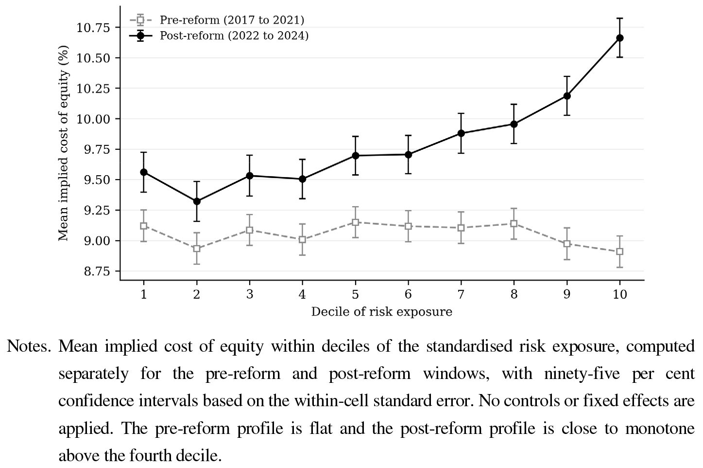
The magnitude in column 4 is 0.313 percentage points per standard deviation of risk exposure, which is 3.4 per cent of the sample mean implied cost of equity. For a firm at the ninetieth percentile of energy intensity located in a spot-pilot province, the implied difference against a median firm is on the order of one percentage point of required return, which is economically material for capital budgeting. [Figure 4] shows the same relation without a functional form assumption. Sorting firm-years into deciles of risk exposure, the mean implied cost of equity is flat across deciles before the reform, with a spread of minus 0.213 percentage points between the top and bottom decile, and monotone after it, with a spread of 1.101 percentage points. Conditioning on both exposures at once tells the same story. Sorting firm-years into the twenty-five cells of the joint quintile grid, the mean change in the implied cost of equity from the pre-reform to the post-reform window rises from 0.280 percentage points in the bottom risk quintile to 1.367 in the top, and the same gradient is present within every populated level-exposure column. Moving across level quintiles the change goes from 0.412 to 0.951, but that movement is not present within a fixed risk row, which is what the regression estimates in <Table 5> formalise.
The level result should be read within the design that produces it. A higher expected electricity price can reach the required return indirectly, through lower profitability, weaker cash flow and higher leverage, and the operating results in Section Ⅳ.3 show that the first of those steps is present in the data. What <Table 5> shows is narrower: conditional on risk exposure, on the lower-order energy-intensity term and on the fixed effects, level exposure has no incremental association with the implied cost of equity in this sample and with this measure. Three readings are consistent with that. The level change may be capitalised in expected cash flows rather than in the discount rate, which is what the framework in Section Ⅱ.3 predicts for an anticipated shift in the mean of an input price. It may reach the discount rate only through channels, such as leverage and profitability, that the control vector holds fixed, in which case the coefficient in <Table 5> is net of those channels rather than evidence that they are absent; re-estimating column 4 without the accounting controls returns a level coefficient of -0.028 (t = -0.27), which does not alter this reading. Or the implied cost of equity may respond to the level with a lag that three post-reform years do not capture. The paper does not distinguish among these, and the statement in the abstract and conclusion that level exposure does not appear in the implied cost of equity is a statement about this design and this measure, not a claim that the price level is irrelevant to financing costs.
<Table 5>
The cost of equity and the two exposures
Notes. The dependent variable is the implied cost of equity in percentage points. Columns (2) to (6) include the lower-order EI x Post term. Column (4) is the preferred specification with firm, industry-by-year, and province-by-year fixed effects. Column (5) constructs the provincial exposure using 2022 price information only. t-statistics based on province-clustered standard errors are in parentheses. ***, **, and * denote significance at the 1%, 5%, and 10% levels.
2. Dynamics
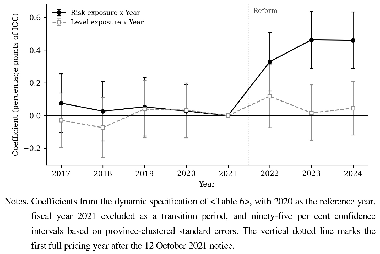
<Table 6> and [Figure 5] report the year-by-year interactions with 2020 as the reference and fiscal year 2021, the transition year, excluded. All three pre-reform risk coefficients lie between minus 0.014 and 0.021 percentage points with t-statistics below 0.3, and the corresponding level coefficients lie between minus 0.052 and 0.024. A joint test that the pre-reform RiskExp and LevelExp interactions are zero returns a p-value of 0.612. The risk coefficient becomes 0.263 in 2022, 0.350 in 2023 and 0.332 in 2024, with t-statistics of 3.24, 4.31 and 4.09. The level coefficients remain indistinguishable from zero throughout the post period. The timing matches the reform and the profile is a level shift rather than a trend, which is consistent with a repricing of a newly variable input. The flat pre-reform profile supports the standard parallel trends assumption of Section Ⅲ.3; it does not by itself establish the stronger assumption required to read the slope in exposure as a marginal causal effect. The 2022 coefficient also deserves a note: the exposure entering it is built from 2022 to 2024 prices, so the year-by-year construction in Section Ⅳ.5, which uses only settlement months observed up to each year, is the appropriate check on whether the 2022 estimate reflects information available in 2022.
<Table 6>
Dynamic specification
Notes. The dependent variable is ICC. The reference year is 2020. Fiscal year 2021 is treated as a transition period and excluded from the primary event-study estimation. The joint pre-reform test for the RiskExp and LevelExp interactions yields p = 0.612. All specifications include the full control vector reported in <Table 5>.
3. Where the Level Shock Goes
<Table 7> turns to the real side. Level exposure is associated with gross margins lower by 1.036 percentage points, with a t-statistic of minus 6.21, while the risk coefficient is minus 0.181 and is not distinguishable from zero at conventional levels. Level exposure is associated with energy intensity lower by 0.291 percentage points and with energy-saving patent applications higher by 0.021 log points, both with t-statistics above 3.7. Firms with greater level exposure show lower energy intensity, more energy-saving applications and lower margins after the reform. This is the response the prior literature reports, and recovering it here is a validation of the level exposure rather than a new finding.
The risk exposure sorts differently. It is associated with cash-flow volatility higher by 0.223 percentage points, with a t-statistic of 5.18, and with capital expenditure lower by 0.281 percentage points, with a t-statistic of minus 4.73. It is the variability of the input price, not its level, that is associated with the volatility of realised cash flow and with capital expenditure.
The final column of <Table 7> adds cash-flow volatility to the cost-of-equity specification. The risk coefficient falls from 0.313 to 0.205. The attenuation is consistent with realised cash-flow volatility being one channel through which the exposure reaches the discount rate, but a comparison of coefficients across specifications does not identify a mediated effect. Cash-flow volatility is itself an outcome of the firm’s risk environment, and any omitted factor that raises both it and the required return produces the same attenuation. The attenuation is what H3, stated as a prediction about a coefficient rather than about mediation, requires. We read H3 as supported in that limited sense, and we do not assign a share of the association to the channel.
<Table 7>
Real-side outcomes and the cash-flow volatility channel
Notes. Columns (1) to (5) report exposure regressions for operating outcomes. Column (6) adds CFVol to the preferred ICC specification. All models include EI x Post, the full control vector, firm fixed effects, industry-by-year fixed effects, and province-by-year fixed effects. t-statistics based on province-clustered standard errors are in parentheses.
4. Cross-sectional Variation
<Table 8> splits the sample. Among firms that do not disclose a long-term bilateral power purchase contract the risk coefficient is 0.343 with a t-statistic of 4.31; among firms that do it is 0.206 with a t-statistic of 2.38. The interaction coefficient in the pooled specification is minus 0.216 with a t-statistic of minus 3.08. Firms disclosing long-term contracts show an association roughly two-fifths weaker, which is consistent with H4. The indicator records whether a contract is disclosed and not the volume covered or the degree to which the price is fixed, and contract adoption is a choice, so the split describes an observed difference between disclosing and non-disclosing firms rather than an effect of hedging. The pattern is the one a hedging interpretation requires, but it does not establish that interpretation, and the notes to <Table 8> and the conclusion state the result at that level.
Self-generation capacity is associated with a smaller point estimate, 0.284 against 0.322, but the interaction is not distinguishable from zero. State ownership does not sort the association, with coefficients of 0.318 and 0.303 in the two subsamples. Financial constraint, measured by the SA index, does not sort it either. The absence of an ownership gradient is worth noting, since a political-insurance interpretation of state ownership would have predicted one.
Panel B of <Table 8> reports three further splits. The first asks whether the risk association is a feature of the administratively designated energy-intensive industries, which the 2021 notice exempted from the upward twenty per cent limit and which therefore faced the widest price distribution, or of energy-intensive firms wherever they are located. If the association were driven by the exemption alone, it should be confined to the listed industries. The risk coefficient is 0.348 (t = 3.76) among firms in the listed industries and 0.292 (t = 3.21) among the remainder, and the triple interaction is 0.061 (t = 0.64). The association is present in both groups, so the pricing of variability is not confined to the exempted industries; the larger coefficient in the listed group is consistent with the removal of the ceiling widening the distribution those firms face, although the difference between the two groups is not statistically distinguishable from zero. Section Ⅳ.6 makes the same point from the other direction: the industry indicator adds nothing once the continuous exposures are included, and half of the variation in risk exposure lies within industries.
The second split concerns local tariff relief. Many manufacturing and strategic emerging-industry firms receive preferential tariffs or fiscal subsidies from local governments, and a firm whose effective tariff is held down by such relief is less exposed to the marketised price than its energy intensity implies. Relief that is stable within a firm over the sample is absorbed by the firm fixed effects, and relief that varies at the province-year level, as provincial tariff programmes do, is absorbed by the province-by-year effects, so what remains is relief that changed at the reform differentially for high-intensity firms. Two specifications address it. The first adds the ratio of government subsidies received to total assets, and its interaction with Post, to the control vector; the risk coefficient is 0.308 (t = 3.96). The second splits the sample at the pre-reform median of that ratio: the risk coefficient is 0.352 (t = 4.18) among low-subsidy firms and 0.271 (t = 3.09) among high-subsidy firms, with a triple interaction of -0.076 (t = -0.88). The somewhat weaker association among heavily subsidised firms is consistent with relief dampening exposure and implies that the baseline, if anything, understates the association for unsubsidised firms; the difference between the two groups is not statistically distinguishable from zero, so relief does not account for the result. Disclosed subsidies capture fiscal transfers rather than negotiated tariff discounts, so the test is indirect, and the fixed-effect argument carries the remaining weight.
The third split bears on what the risk exposure measures. RiskExp is the product of a firm’s energy intensity and the realised volatility of its provincial price, so it is high for energy-intensive firms in volatile provinces and low both for energy-intensive firms in stable provinces and for low-intensity firms anywhere. The lower-order term EI × Post absorbs any post-reform change common to energy-intensive firms in every province, including a general increase in the uncertainty such firms face after marketisation, and the industry-by-year effects absorb uncertainty common to an industry in a year. The coefficient on RiskExp × Post is therefore identified from the difference in post-reform changes between energy-intensive firms located in more and less volatile provinces, holding the province-wide change fixed, which is what distinguishes exposure to the variability of the electricity price from a general exposure of energy-intensive firms to uncertainty. The randomisation inference in Section Ⅳ.5, which permutes the provincial moments across provinces, tests the same distinction: if the coefficient reflected energy-intensive status rather than the provincial price process, reassigning provinces’ moments would leave it unchanged, and it does not. The pilot-status split in Panel B makes the point without using realised prices: the risk coefficient is 0.367 (t = 4.11) in the fourteen pilot provinces and 0.244 (t = 2.61) elsewhere. What the design cannot exclude is a provincial shock that raised both price volatility and other sources of uncertainty for energy-intensive firms in the same provinces after 2022; the paper reads the coefficient as the association with the provincial price process, of which realised volatility is the measured component.
<Table 8>
Cross-sectional variation in the risk association
Notes. Each pair of columns reports split-sample estimates. The triple-interaction coefficient is estimated in the pooled sample. All models include the complete control vector listed in <Table 5> and the lower-order terms required by the interaction structure. The LTC result is associative because contract adoption and coverage are not randomly assigned, and the indicator records disclosure of a contract rather than the volume or price covered. Panel B splits the sample by membership of the administrative energy-intensive industry list, by the pre-reform median of government subsidies received scaled by total assets, and by spot-market pilot status of the headquarters province as designated in August 2017 and April 2021.
5. Sensitivity
This section organises the robustness evidence by the methodological concern each exercise addresses, and <Table 9> reports the estimates in the same order. Four concerns are relevant: the use of realised post-reform prices in the exposure, the measurement of the exposure weight, inference with thirty-one provincial clusters, and functional form together with the measure of the dependent variable.
Future information in the exposure. The baseline provincial moments are computed from settlement prices realised over 2022 to 2024, so the exposure assigned to a firm-year in 2022 contains information that was not available in 2022. Column 5 of <Table 5> restricts the moments to 2022 settlement months and returns 0.262 (t = 3.44); this removes the 2023 and 2024 information but still uses prices realised during 2022 itself, so it is a check on whether the later years drive the estimate rather than a fully ex-ante measure. Two further constructions complete the exercise. The first rebuilds both exposures separately for each post-reform year from the settlement months observed up to and including that fiscal year, so that the 2022 exposure uses 2022 months only, the 2023 exposure uses 2022 and 2023 months, and so on; the risk coefficient is 0.297 (t = 3.76). The second is a supplementary analysis that uses pre-reform spot-market pilot status, announced before the reform, in place of realised prices as the source of cross-provincial variation. In reduced form, EI × Pilot × Post enters in place of RiskExp × Post and returns 0.274 (t = 3.30); when the pilot designation interacted with EI and Post is used to instrument RiskExp × Post, the first-stage F-statistic is 18.7 and the second-stage coefficient is 0.341 (t = 3.04). This exercise is read as a complement to the year-by-year construction rather than as a separate identification strategy: the pilot designation is a coarse proxy for variability, it does not remove the concern about post-reform information on its own, and the reduced-form coefficient is not directly comparable in magnitude to the baseline. What it shows is that a measure investors could have held in 2021 produces the same sign and a comparable statistical strength.
Measurement of the exposure weight. EI combines electricity with fuel cost. Restricting the sample to the 1,024 firms that disclose purchased electricity separately and rebuilding both exposures from the electricity-only item returns a risk coefficient of 0.336 (t = 3.57) against 0.318 (t = 3.41) for the combined measure on the same subsample. Adding classical measurement error to pre-reform EI retains 95.5 per cent of the preferred coefficient when the noise standard deviation equals one-quarter of the cross-sectional standard deviation, and 88.8 per cent when it equals one-half, which is the attenuation one expects if the fuel component behaves as noise. Orthogonalising level exposure against risk exposure leaves the risk coefficient at 0.431 and the orthogonalised level coefficient at 0.044, and reversing the orthogonalisation still produces a risk coefficient of 0.254, significant at the 0.1 per cent level, so the separation of the two moments does not depend on which is given priority.
Inference. The preferred estimate is 0.313 with a province-clustered standard error of 0.078 (t = 4.02). Given only thirty-one provincial clusters, small-cluster inference follows Cameron et al. (2008), and the wild cluster bootstrap yields p < 0.001. Randomisation inference, based on permuting the provincial premium and volatility measures across provinces and reconstructing both exposures, produces a placebo distribution centred at -0.006 with a standard deviation of 0.098, and the actual coefficient lies in the upper tail with p = 0.004. A placebo reform dated to 2019 using only pre-reform years yields -0.028 (t = -0.49), and one dated to 2020 yields 0.019 (t = 0.46), so no corresponding pre-existing differential trend is present.
Functional form and the dependent variable. Using the PEG, residual-income and Claus and Thomas measures separately yields risk coefficients of 0.371, 0.385 and 0.362, so the result does not depend on which implementation of the implied cost of equity is used. Excluding utilities and petroleum processing firms gives 0.399, and excluding 2020 gives 0.379. Replacing the linear exposure with quintile indicators interacted with Post returns coefficients of 0.108, 0.224, 0.361 and 0.512 for the second to fifth quintiles relative to the first, increasing monotonically across the distribution, which is the pattern [Figure 4] shows without controls and which indicates that the linear coefficient is not produced by a small group of extreme firms.
<Table 9>
Sensitivity of the risk association
| Estimate | SE / SD | t / p | Concern addressed | |
|
A. Future information in the exposure | ||||
|
Preferred RiskExp x Post (2022 to 2024 moments) | 0.313 | 0.078 | t = 4.02 | Benchmark |
|
2022 moments only (<Table 5>, column 5) | 0.262 | 0.076 | t = 3.44 |
Removes 2023 and 2024 information |
|
Year-by-year moments, months to year t | 0.297 | 0.079 | t = 3.76 |
Uses no information beyond each year |
|
Supplementary: EI x Pilot x Post (pre-reform pilot status) | 0.274 | 0.083 | t = 3.30 |
Pre-reform designation; complements, does not replace, Panel A |
|
Supplementary: RiskExp x Post, pilot-based specification | 0.341 | 0.112 | t = 3.04 | First-stage F = 18.7 |
|
B. Measurement of the exposure weight | ||||
|
Electricity-only EI, disclosing subsample | 0.336 | 0.094 | t = 3.57 |
Combined EI on same subsample: 0.318 |
|
EI measurement-error sensitivity (25%) | 0.299 | 0.079 | t = 3.78 |
95.5% of preferred coefficient retained |
|
EI measurement-error sensitivity (50%) | 0.278 | 0.081 | t = 3.43 | 88.8% retained |
|
Level orthogonalised against risk | 0.431 | 0.090 | t = 4.79 |
Orthogonalised level coefficient 0.044 |
|
Risk orthogonalised against level | 0.254 | 0.071 | t = 3.58 | Significant at 0.1% |
| C. Inference | ||||
| Wild cluster bootstrap | 0.313 | p < 0.001 | 31 provincial clusters | |
| Randomisation inference | 0.313 | 0.098 | p = 0.004 |
Placebo distribution mean = -0.006 |
| Placebo reform in 2019 | -0.028 | 0.057 | t = -0.49 | Pre-reform years only |
| Placebo reform in 2020 | 0.019 | 0.041 | t = 0.46 | Pre-reform years only |
|
D. Functional form and dependent variable | ||||
|
ICC_PEG / ICC_GLS / ICC_CT |
0.371 / 0.385 / 0.362 | Alternative ICC implementations | ||
|
Excluding utilities and petroleum processing | 0.399 | 0.087 | t = 4.59 | Sector composition |
| Excluding 2020 | 0.379 | 0.084 | t = 4.51 | Pandemic year |
|
Risk exposure quintiles Q2 to Q5 x Post |
0.108 / 0.224 / 0.361 / 0.512 |
Relative to Q1; no linearity assumption |
Notes. All reported specifications include the full control vector, EI x Post, and the preferred fixed effects unless otherwise stated. Panel A varies the information set used to construct the provincial moments; the pilot designation is the spot-market pilot status announced in August 2017 and April 2021, and the two pilot-based rows are supplementary analyses rather than a separate identification strategy. Panel B varies the exposure weight. Panel C varies the inference procedure. Panel D varies the functional form and the implementation of the implied cost of equity; the estimates for the alternative ICC measures, the sample exclusions and the orthogonalised exposures are re-estimated under the preferred fixed-effect structure. Standard errors are clustered by province.
6. Comparison with the Industry-List Design
<Table 10> directly compares the conventional industry-list design with the continuous-exposure approach. Using firms covered by the administrative energy-intensive industry classification as the treated group yields a post-reform coefficient of 0.631 percentage points (t = 7.95), which on its own would be read as a sizeable post-reform difference between listed and other industries. In the same sample, however, the continuous-exposure specification produces a risk coefficient of 0.313 (t = 4.02) and a level coefficient of -0.050. When the industry indicator and both exposures enter jointly, the industry coefficient falls to 0.007 (t = 0.06), while the risk coefficient remains 0.309 (t = 3.91). Thus, once exposure is measured directly, the industry indicator contributes little additional information, and most of the association is attributed to price variability rather than price level. This is consistent with recent evidence that difference-in-differences estimands depend on the distribution of treatment intensity and that exposure-weighted and binary designs identify different objects (de Chaisemartin and D’Haultfœuille, 2020; Callaway and Sant’Anna, 2021; Goodman-Bacon, 2021; Sun and Abraham, 2021; Borusyak et al., 2022; Callaway et al., forthcoming). Two additional exercises explain why the industry list performs poorly. The risk-exposure distributions of listed and non-listed firms overlap substantially. Among firms in the top quintile of risk exposure, 25.2 per cent fall outside the administrative list, while 30.8 per cent of listed firms fall below the same threshold. The binary classification therefore misclassifies firms in both directions. The variance decomposition leads to the same conclusion. Removing industry means leaves 50.6 per cent of the variance in risk exposure and 54.5 per cent in level exposure, while removing provincial means leaves 90.5 and 89.3 per cent, respectively. Removing both leaves 30.8 and 31.6 per cent. Hence, roughly half of the relevant exposure variation occurs within industries and is lost in an industry-level treatment design, whereas most variation survives the removal of provincial means, allowing the continuous exposures to remain identified even with province-by-year fixed effects.
<Table 10>
This design against the industry-list design
Ⅴ. Conclusion
China’s October 2021 coal-power tariff reform simultaneously changed the level and variability of an unavoidable industrial input price, with the two changes displaying largely distinct cross-provincial patterns. Separating these dimensions shows that variability exposure has the larger and more consistent association with the implied cost of equity, whereas level exposure is indistinguishable from zero in this design once the lower-order energy-intensity term is included. The latter instead appears in operating outcomes, including margins, energy intensity and energy- saving innovation. The risk coefficient is attenuated when realised cash-flow volatility is controlled for, and the association is weaker among firms disclosing long-term bilateral power contracts; both patterns are consistent with cash-flow volatility and contractual hedging as relevant mechanisms without establishing either. The association survives when the exposure is rebuilt from 2022 prices alone, from the months observed up to each year, or from the spot-pilot designation announced before the reform, and it is present outside the administratively designated energy-intensive industries as well as within them.
These findings imply that evaluating price marketisation solely through changes in average prices is incomplete. A predictable increase in tariffs and an unchanged but more variable tariff have different implications for the cost of capital, and it is the second that is associated with the required return in this setting. The policy instruments that bear on that second dimension already exist in the Chinese market design, and the results speak to how they are calibrated. First, the medium- and long-term contracting requirements that the National Development and Reform Commission attaches to each contracting year, which for 2023 required market users to cover at least eighty per cent of the previous year’s consumption with annual contracts and ninety per cent with contracts of all horizons, are the direct counterpart of the hedging split in <Table 8>: the weaker association among contracting firms suggests that coverage requirements, and the contract-for- difference arrangements into which priority generation is being converted in the spot pilots, act on the dimension of the price that the equity market prices. Second, the coal-price linkage clauses that the same notices encourage shift variability from the electricity price to the fuel price and do not remove it, so their value for the cost of capital depends on whether the firm can hedge the linked index. Third, the grid-company agency purchasing mechanism introduced alongside the 2021 reform, under which users not yet trading directly are served at a monthly announced price, sets the variability that smaller industrial users face; the evidence here suggests that the frequency at which that price is reset is a cost-of-capital parameter and not only a pass-through parameter. Fourth, the settlement information that provincial trading centres publish is what allows a firm and its investors to measure the exposure at all, and the near-orthogonality of the level and variability of the premium across provinces means that a disclosure regime that reports only average prices would leave the priced dimension unobserved. For markets in which industrial tariffs remain administered and marketisation is under discussion, including Korea, the sequencing of hedging infrastructure relative to price liberalisation is a first-order design choice on this evidence rather than a detail of implementation.
The limitations of the study attach to specific results rather than to the design as a whole. The provincial moments are built from prices realised over 2022 to 2024, so the 2022 exposure in <Table 5> and the 2022 coefficient in <Table 6> contain information not yet available in that year; the estimates in <Table 9>, Panel A, which use 2022 months only, months up to each year, or the pre-announced pilot designation, indicate that this construction is unlikely to generate the association, with the pilot-based specifications read as supplementary checks rather than as a separate identification strategy, and the paper treats the baseline exposure as a description of the post-reform regime rather than of contemporaneous expectations. The exposure weight combines electricity with fuel cost, so the level and risk exposures are energy-cost rather than electricity-only exposures; the electricity- only re-estimation and the measurement-error exercise in <Table 9>, Panel B, bound what that costs, and the operating results for energy intensity in <Table 7> should be read as results for the combined item. The implied cost of equity is model based and inherits the properties of analyst forecasts; the three implementations in <Table 9>, Panel D, agree in sign and magnitude, and Appendix B documents the choices on which they rest, but a measure that responds to the price level with a longer lag than three years would not be detected here. The long-term contract indicator records disclosure rather than contracted volume, and disclosure is a choice, so the result in <Table 8> concerns the presence of a contract and is associative. Finally, because exposure is continuous, the preferred coefficient of 0.313 is the post-reform difference between firms one standard deviation apart in exposure under the standard parallel trends assumption, and reading it as the effect of a marginal change in exposure requires the stronger assumption discussed in Section Ⅲ.3, which the pre-reform evidence cannot test.
