

Ⅰ. Introduction
Ⅱ. Literature Review
Ⅲ. Data and Estimation Approach
1. Data
2. Econometric Model
3. Climate Change Scenarios
4. Carbon Costs Analysis
Ⅳ. Estimation Results
1. Unit root and bound tests results
2. Estimation results of the ARDL Error Correction Model
3. Application of the SSP and NGFS scenarios
Ⅴ. Conclusion and Policy Implication
1. Summary
2. Policy implications
Ⅵ. Limitations of the Study
◎ Appendix ◎
Ⅰ. Introduction
Climate change has emerged as one of the most pressing global challenges, with far-reaching consequences for ecosystems, human livelihoods, and economic stability. According to the Intergovernmental Panel on Climate Change (IPCC) Sixth Assessment Report (IPCC, 2023), global surface temperatures increased by 1.09°C above pre-industrial levels between 2011 and 2020. If greenhouse gas (GHG) emissions continue at their current levels, global warming is likely to surpass the critical threshold of 1.5°C as early as 2021-2040 (Korea Meteorological Administration, 2023). Rising temperatures drive extreme weather events, disrupt infrastructure, and increase energy demand.
South Korea is particularly vulnerable to the economic impacts of climate change. Over the past decade (2013-2023), climate-related disasters have resulted in economic damages estimated at KRW 4.1 trillion, with recovery costs exceeding KRW 11.8 trillion, culminating in total economic losses of KRW 15.9 trillion (Lee 2024). However, this figure accounts only for the financial impact of natural disasters (e.g., floods, heavy rainfall, heavy snowfall, and droughts) and provides only a partial economic measure of climate change effects. Academic research has increasingly analyzed the economic impact of climate change on regional economies, particularly by estimating economic losses using climate variables such as temperature and precipitation under different Shared Socioeconomic Pathway (SSP) scenarios and assessing damage costs in industries vulnerable to climate change.
Extreme temperature anomalies caused by climate change significantly increase the volatility of electricity consumption. The relationship between temperature and electricity demand follows a fundamental pattern: electricity consumption rises asymmetrically beyond a critical temperature threshold. Heatwaves and cold waves, in particular, lead to sharp increases in electricity demand (Park and Seo, 2019). Rising temperatures drive increased cooling demand, while fluctuations in seasonal temperatures influence heating needs, demonstrating that extreme temperatures have a direct impact on electricity consumption. Additionally, socio-demographic shifts, such as the increasing prevalence of single-person households, further compound energy consumption patterns (Kim, 2021).
The primary objective of this study is to investigate the determinants of residential electricity consumption in Gwangju Metropolitan City (hereafter, Gwangju), with a particular focus on climate-related variables. The residential sector in Gwangju plays a critical role in its energy landscape, accounting for approximately 25% of total electricity consumption. Using an Autoregressive Distributed Lag (ARDL) model, this study analyzes long-term relationships between electricity consumption and key explanatory variables, including average temperature, precipitation rate, share of single-person households, cooling degree days (CDD), and heating degree days (HDD). Moreover, we consider a non-linear relationship between average temperature and electricity consumption. In the next step, the study employs Shared Socioeconomic Pathway (SSP) scenarios, from Gwangju Metropolitan City Climate Change Outlook Report (Korea Meteorological Administration, 2023), to estimate scenario-based future electricity demand due to climate change and assess the economic implications of increased CO2 emissions using the Network for Greening the Financial System (NGFS) carbon pricing framework.1) By integrating localized data with established climate scenarios, this research provides valuable insights to inform energy policy, urban planning, and climate adaptation strategies for Gwangju and other similar urban inland regions.
The remainder of this paper is structured as follows. Section 2 reviews the existing literature on the impact of climate change on electricity consumption and economic activity. Section 3 details the data sources and methodology, outlining the econometric approach used in this study. Section 4 presents the empirical results, including scenario-based estimations of future residential electricity demand, CO2 emissions, and associated carbon costs. Section 5 concludes with a summary of the main findings and discusses their policy implications. Finally, Section 6 outlines the study’s limitations and offers suggestions for future research.
Ⅱ. Literature Review
In recent years, a growing body of research has examined the economic impacts of climate change. For instance, Tol (2024) conducted a meta-analysis of 39 studies and concluded that the central estimate of global warming’s economic impact remains consistently negative, although the confidence interval has widened compared to previous analysis (Tol, 2019). This broader range reflects the potential positive effects of climate change, such as reduced heating costs in winter, lower cold-related mortality, and carbon dioxide fertilization (Desmet and Rossi-Hansberg, 2015; Newell et al., 2021). However, both meta-analyses (Tol, 2019, 2024) found that uncertainty about climate change impacts is skewed toward negative outcome, with poorer countries being significantly more vulnerable than wealthier nations. Given the geographical variation in climate change effects, this section focuses on studies related to South Korea.
Several studies have examined the relationship between temperature and electricity consumption, highlighting the significant impact of temperature fluctuations on energy demand. For example, Lee and Hong (2010) analyzed Korea’s sensitivity of electricity supply and demand to temperature change in different urban areas and found that extreme weather events driven by climate change have altered seasonal electricity demand patterns. In January 2021, a severe cold wave caused winter peak electricity demand to surpass summer peak demand, marking a significant shift in consumption trends. Their findings suggest that temperature variations influence electricity demand throughout the year, rather than being confined to a specific season. Furthermore, their study showed that commercial buildings exhibit greater temperature sensitivity than residential buildings. Similarly, Kim et al. (2015) estimated Korean electricity demand function incorporating quarterly data on average temperature, GDP, electricity prices, and electricity consumption from 2005 to 2013. Their results, based on an instrumental variable approach, confirmed that both income elasticity and price elasticity significantly influence long-term electricity demand, while the relationship between electricity consumption and temperature follows a U-shaped pattern.
Jeong and Heo (2015) incorporated heating and cooling degree days as key explanatory variables in electricity demand analysis. Applying an Autoregressive Distributed Lag (ARDL) model, they assessed the impact of climate change on heating and cooling demand in Seoul from 1995 to 2014. Their findings indicated that both heating and cooling degree days were statistically significant determinants of electricity consumption, with cooling degree days playing a more critical role. Yoo and Won (2022) used a panel analysis to examine summer residential electricity consumption and found that both higher cooling degree days and increased income levels contributed to greater electricity usage.
Another stream of literature has examined the impact of demographic changes on electricity demand. Studies suggest that household size and composition influence energy consumption patterns, with single-person households exhibiting higher per capita energy use compared to multi-person households (Kim, 2021). Seo et al. (2009) analyzed variations in electricity usage according to household size, income level, housing size, and heating energy type. The study found that single-person households showed the highest per capita energy consumption. Similarly, Kim et al. (2011) analyzed energy consumption patterns in detached houses and reported the highest per capita energy use among single-person households. Lee (2024) analyzed the correlation between population aging and residential electricity consumption using panel data, incorporating the proportion of single-person households to reflect demographic, economic, and climate-related factors. Thus, the inclusion of the share of single-person households is particularly relevant for Gwangju, where this demographic has been steadily increasing (from 16% in 2002 to 34% in 2022, and is projected to reach 40% by 2050), potentially leading to significant shifts in residential electricity demand.
In the broader context of urban energy transitions, several studies have investigated how the diffusion of renewable energy contributes to climate change mitigation and may influence future electricity demand patterns. For example, Bae and Jung (2020) employed a panel econometric model to assess whether the expansion of renewable energy led to reductions in air pollutants, including particulate matter, and identified notable regional disparities in the effectiveness of these measures. Lim (2023) examined the economic ripple effects of replacing thermal power plants with renewable sources under four scenarios, analyzing changes in greenhouse gas emission inducement coefficients, production inducement coefficients, and value-added inducement coefficients. These findings underscore the evolving structure of urban energy systems and the importance of integrating renewable energy development into long-term electricity demand forecasting.
Scenario-based modeling has also become central in assessing future energy demand under different socio-economic and policy conditions. The Shared Socioeconomic Pathways (SSPs) framework offers a comprehensive basis for such projections. For example, Choi et al. (2024) estimated that, under current climate policy conditions, direct climate damage in Busan could increase by 2.7 times over the next decade. Additionally, NGFS scenarios have been widely applied to assess economic impacts from climate-induced changes. Cho and Min (2024), for instance, used NGFS carbon price scenarios to estimate long-term effects on agricultural and consumer prices.
The COVID-19 pandemic also temporarily influenced residential electricity demand. Studies such as Krarti and Aldubyan (2021) and Li et al. (2021) reported increases in New York City’s residential electricity usage ranging from 15% to 53% compared to pre-pandemic levels. However, Jang et al. (2021) and Kang et al. (2021) found that the impact in Korea was considerably smaller than in other countries and short-lived.
While extensive research has explored the links between temperature and electricity demand, relatively few studies have estimated the economic costs of carbon emissions resulting from increased residential electricity consumption, especially in the context of an inland metropolitan area like Gwangju. A study by the Ministry of Environment and Korea Environment Institute (2022) projected changes in monthly electricity consumption per household and commercial contract unit under climate change scenarios. Using SSP-based projections, the analysis found that both residential and commercial electricity use will increase over time, with greater variation depending on the emissions pathway. Under the low- emissions SSP1-2.6 scenario, long-term increases were estimated at 0-6% for households and 0-5% for commercial users. In contrast, under the high-emissions SSP5-8.5 scenario, household electricity consumption could rise by 4-25%, and commercial use by 2-15% in the long term. The broader and higher variability in the SSP5-8.5 scenario reflects increasing uncertainty in climate models and temperature divergence among model projections over time. These national-level findings support the importance of localized analyses, such as the present study of Gwangju, in understanding climate-induced shifts in electricity demand, thereby contributing to the growing literature on climate change and energy economics.
Ⅲ. Data and Estimation Approach
1. Data
This study uses monthly time series data from January 2002 to December 2022 for Gwangju Metropolitan City. Electricity use in the residential sector is the dependent variable. The paper considers five main explanatory variables influencing electricity use: average temperature, precipitation, the share of single-person households, CDD, and HDD. We also tested the inclusion of monthly dummy variables to control for seasonal effects; however, due to strong multicollinearity with temperature-related variables (average temperature, CDD, and HDD), these dummies were excluded from the final model specification.
Cooling and heating degree days (CDD and HDD) were computed using reference temperatures of 24°C for cooling and 18°C for heating, respectively. The share of single-person households is defined as the ratio of the number of single-person households to the total number of households in Gwangju for each respective year. This variable is included to capture the influence of household structure on residential electricity consumption. We posit that the prevalence of single-person households plays a significant role in shaping energy demand, as such households typically require essential home appliances regardless of household size. Consequently, an increase in the share of single-person households is expected to contribute to higher aggregate residential electricity use.
Data on average temperatures and precipitation were obtained from the Korea Meteorological Administration Weather Data Service.2) Information on electricity use in the residential sector was collected from Electric Power Data Open Portal System.3) Data on CDD and HDD were sourced from the Public Data Portal,4) while data on the number of single-person households and total number of households were obtained from KOSIS (Korean Statistical Information Service) Statistics.5)
For the analysis, logarithmic transformation was applied to electricity use and precipitation. This transformation addresses scalability issues and simplifies the interpretation of coefficient estimators as demand elasticities. However, CDD, HDD, and average temperature were not log-transformed due to the presence of zero and negative values. Moreover, the share of single-person households is included in levels rather than log-transformed, as it is expressed as a percentage, applying a logarithmic transformation would complicate interpretation without offering meaningful improvements in model specification.
To address potential nonlinearity in the relationship between temperature and electricity use, following Lee and Chiu (2011) and Kim et al. (2015) we include a squared temperature term in the model. This allows for estimation of elasticity at different temperature levels, and in particular enables comparison of point elasticities around temperature thresholds of interest (e.g., mean seasonal values).
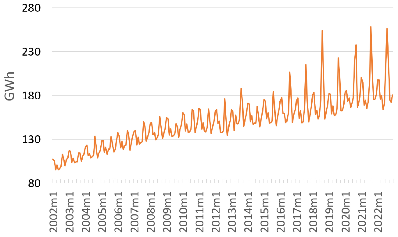
[Figure 1] illustrates the trend in electricity use in the residential sector. The figure shows a clear increasing trend in electricity consumption. Specifically, annual electricity uses in the residential sector rose from 1,237.5 GWh in 2002 to 1,802.7 GWh in 2022. <Table 1> provides descriptive statistics for the dataset.
<Table 1>
Descriptive Statistics of Key Variables
2. Econometric Model
The study employs the Autoregressive Distributed Lag (ARDL) model to analyze the short- and long-run elasticities of residential electricity consumption in response to climatic and demographic variables. This model is well-suited for datasets where variables are integrated of order I(0) and I(1). While the ARDL- ECM framework does not endogenously model structural energy system feedbacks (as in integrated models like Global Change Analysis Model, GCAM), it allows for transparent, empirical estimation of climate sensitivity and demographic effects on electricity demand. These elasticity estimates are valuable inputs for broader scenario-based planning and modeling frameworks. The ARDL model also allows for flexible lag structures, making it particularly effective in capturing the temporal dynamics among variables.
The general form of the ARDL model is as follows:
Where, yt is a dependent variable, xt is a set of explanatory variables, c0 is an intercept, p and q are lag orders, and are estimated parameters, ut and is the regression error term. The data are observed at consecutive time points t = 1, 2, …, T.
When analyzing long-term relationships, the ARDL model can be extended into an Error Correction Model (ECM). The ECM is based on the concept of cointegration, which applies when two or more variables move together over time, sharing a common trend. The ARDL-ECM model includes an error correction term that represents the speed at which the system adjusts toward long-term equilibrium, incorporating both short-term dynamics and long-term equilibrium relationships. The general equation of the ARDL-ECM is as follows (Hassler and Wolters, 2006):
In Eq. (2), the coefficient α plays a crucial role as it represents the speed of adjustment, indicating how quickly yt returns to its long-run equilibrium after a disturbance. If α = 1, deviations from equilibrium are fully corrected in the following period, with no additional short-run fluctuations. Conversely, if α = 0, the process never reverts to equilibrium. Values between these extremes indicate a partial adjustment process, where the gap to equilibrium gradually closes over time. To establish the existence of a long-run relationship, two conditions must be satisfied: long-run coefficient is not equal to zero () and .
The coefficients in Eq. (2) can be mapped in a straightforward algebraic way to the coefficients in Eq. (1):
Lags play a crucial role in ARDL estimation. While more lags improve the regression fit, they also increase the variance of coefficient estimates. Akaike information criterion (AIC) or the Schwarz/Bayesian information criterion (BIC) can help balance this trade-off by selecting the optimal lag.
The specific ARDL-ECM model used for estimating electricity consumption is presented in Eq. (4).
Where, EC is Electricity use in residential sector, Temp is Average monthly temperature, Precip is Monthly precipitation, Single_HH is Single-person households ratio to total number of households, CDD is Cooling degree days, HDD is Heating degree days, Ln represents a natural logarithm transformation.
1) Stationarity and Cointegration Tests
Although the ARDL model provides flexibility in estimating long-term relationships between I(1) and I(0) variables, there are two restrictions: first, the dependent variable must be an I(1) variable; second, the integration order of explanatory variables must not exceed I(1). To ensure the validity of the ARDL model, we conducted unit root tests for all variables. Following Durmaz (2020), we test for both level stationarity and trend stationarity using Augmented Dickey-Fuller (ADF) tests and the Kwiatkowski-Phillips- Schmidt-Shin (KPSS) test. The optimal lag length for these tests was determined using the ‘varsoc’ command in Stata, with a lag length of 12 selected based on the majority of information criteria. The ADF test evaluates the null hypothesis of a unit root (nonstationarity), whereas the KPSS test assesses the null of trend stationarity. The feasibility to estimate long-term relationships between variables with mixed order of integration distinguishes ARDL from the other cointegration techniques such as the Johansen test, making it a more flexible approach in time series analysis. The bounds testing approach, proposed by Pesaran et al. (2001), is employed to confirm the presence of a long-run relationship among the variables. The test involves comparing the computed F-statistic against critical values to determine if the null hypothesis of no level relationship can be rejected.
3. Climate Change Scenarios
To capture the potential impacts of climate change, this study incorporates Shared Socioeconomic Pathway (SSP) scenarios. These scenarios provide projections for temperature and precipitation changes based on varying degrees of global mitigation efforts and socio-economic developments. Seasonal baseline for the period 2000-2019 serves as reference points to calculate the projected changes under each SSP scenario. The projected changes are then applied to estimate electricity demand using the long-run coefficients derived from the ARDL model.
The SSP scenarios of projections for average temperature change <Table 2> and precipitation rate <Table 3> were obtained from the Gwangju Metropolitan City Climate Change Outlook Report 2023. The standard greenhouse gas pathways in the IPCC Sixth Assessment Report are four scenarios: SSP1-2.6, SSP2-4.5, SSP3-7.0, and SSP5-8.5. Although Korea’s official climate targets—such as net-zero emissions by 2050 and emissions reduction by 40% by 2030—are more aligned with SSP2-4.5 or even SSP1-2.6 pathways, the country’s actual emissions trajectory and continued reliance on fossil fuels as of 2024 more closely align with SSP3-7.0. Accordingly, this study adopts the SSP3-7.0 scenario for all projections. This choice reflects the likelihood that residential electricity consumption patterns would differ significantly under the more stringent climate policies assumed in SSP1-2.6 and SSP2-4.5. In SSP scenario designations, the first number indicates the level of socio-economic efforts for climate change adaptation and mitigation <Table 4>, while the second number represents the radiative forcing projected for the year 2100.
<Table 2>
Baseline and Projected Average Temperature by Season and Scenario in Gwangju Metropolitan City
(Unit: Celsius degree)
<Table 3>
Baseline and Projected Precipitation Rate by Season and Scenario in Gwangju Metropolitan City
(Unit: mm)
<Table 4>
Definitions of the SSP Scenarios
4. Carbon Costs Analysis
The CO2 emissions associated with electricity consumption are calculated using the emission factor of 478.1 kg CO2 per MWh, as provided by the Korea Climate and Environment Network.6) This factor is applied to the change in projected electricity consumption to estimate the seasonal and annual change emissions under SSP3-7.0 scenario.
This study also utilized carbon price projections from the NGFS (Network for Greening the Financial System) scenarios, developed using the GCAM 6.0, specifically for Korean context. Carbon prices are applied to the projected CO2 emissions from electricity consumption in residential sector under SSP scenario to estimate the economic impact associated with climate change. Although there are seven NGFS scenarios <Table 5>, this analysis applies only the projected carbon prices from the ‘Fragmented World’ scenario. This is because the study uses a fixed emissions factor to convert electricity consumption into CO2 emissions, whereas other NGFS scenarios may assume significant variability of emissions factors over time. <Table 6> presents carbon price projections for all NGFS scenarios applicable to Korea.7)
<Table 5>
Definitions of the NGFS Scenarios
Source: NGFS, 2024
<Table 6>
Projected Carbon Prices under Four NGFS Scenarios
(Unit: 2010 KRW)
In the NGFS scenarios, projected carbon prices refer to shadow prices that are endogenously derived within integrated assessment models (IAMs) to satisfy the emissions constraints specified by each scenario (NGFS, 2024). These prices represent the marginal abatement cost required to meet climate targets—such as net-zero CO2 emissions by 2050—and serve as a proxy for the stringency of climate policy. Unlike market-based carbon prices, which are shaped by political and economic conditions, NGFS carbon prices result from model-based optimization that internalizes assumptions about technological availability (e.g., carbon dioxide removal), the timing of policy implementation, and the degree of regional or global coordination. Generally, higher shadow prices indicate more ambitious mitigation pathways involving earlier and stronger policy actions. Therefore, within the NGFS framework, projected carbon prices should not be interpreted as forecasts of market behavior. Rather, they function as internal benchmarks that reflect the policy effort required to limit global warming under a given scenario.
Ⅳ. Estimation Results
1. Unit root and bound tests results
The results of ADF and KPSS tests are summarized in <Table 7>. The dependent variable, the logarithm of residential electricity consumption, provides weak evidence against the unit root hypothesis in the ADF test without a trend, and fails to reject nonstationarity when a trend is included. In contrast, the KPSS test rejects the null of trend stationarity. Both tests confirm stationarity after first differencing, indicating that the series is integrated of order one, I(1).
For the average temperature variable, the ADF test suggests stationarity at the 10% level with and without a trend, while the squared term does not reject the null of a unit root. KPSS results show that both variables are trend stationary. Based on these findings, both variables are treated as at most I(1).
In the case of the logarithm of precipitation, the ADF test results indicate nonstationarity in both level and trend specifications. Although KPSS statistics fall below the critical values for both level and trend stationarity—suggesting potential stationarity—the preponderance of evidence, especially from the ADF test, supports treating the series as I(1). Stationarity is clearly confirmed after first differencing.
Heating Degree Days (HDD) and Cooling Degree Days (CDD) present mixed results in levels. The ADF test identifies CDD as stationary, while the KPSS test does not. HDD is found to be nonstationary when a trend is included. However, both variables are confirmed to be stationary in their first differences.
The single-person household ratio is nonstationary in levels, but the ADF test rejects the unit root hypothesis when a trend is included, suggesting trend stationarity. The KPSS test provides moderate support for this conclusion. After first differencing, both tests confirm stationarity.
While including a deterministic linear trend in the long-run equation is theoretically warranted to capture potential trend-stationarity in climatic and demographic variables, its practical implementation resulted in severe multicollinearity issues. Specifically, the inclusion of the trend variable led to very high Variance Inflation Factors (VIFs), particularly between trend variable and the single-person household ratio, with VIF values exceeding 170. Moreover, when the trend was included in the ARDL specification, Stata omitted the variable due to perfect collinearity in some model configurations.8) These results indicate that the linear trend is highly correlated with key explanatory variables, and its inclusion could distort parameter estimates and inference. Therefore, despite its theoretical relevance, the deterministic trend was excluded from the final model specification to ensure estimation stability and avoid multicollinearity bias.
<Table 7>
Unit Root Tests Results (ADF and KPS tests, with 12 lags)
| Variable | Test | Level | Trend | First difference |
| Log Electricity Use | ADF | -2.723* | -2.867 | -7.337*** |
| KPSS | 1.950** | 0.360** | 0.0547 | |
| Average temperature | ADF | -2.641* | -3.136* | -9.588*** |
| KPSS | 0.445** | 0.138* | 0.269 | |
| Average temperature square | ADF | -2.470 | -2.974 | -9.055*** |
| KPSS | 0.450** | 0.140* | 0.221 | |
| Log Precipitation rate | ADF | -1.528 | -1.928 | -9.422*** |
| KPSS | 0.267 | 0.0888 | 0.0466 | |
| HDD | ADF | -2.911** | -3.032 | -14.080*** |
| KPSS | 0.552** | 0.218** | 0.236 | |
| CDD | ADF | -3.709*** | -3.893*** | -15.177*** |
| KPSS | 0.418** | 0.125* | 0.104 | |
| Single-person Households Share | ADF | -0.289 | -3.746*** | -3.464*** |
| KPSS | 2.030** | 0.102 | 0.0463 |
Overall, all variables are found to be either I(0), I(1), or trend-stationary, with no indication of I(2) behavior. This satisfies the key requirement for the ARDL bounds testing approach and justifies proceeding with the ARDL-ECM estimation framework.
The ARDL bound test results confirm a long-term relationship between variables (<Table 8>). Specifically, the estimated F-statistic (45.659) exceeds the upper critical value (4.43) at the 1% significance level, leading to the rejection of the null hypothesis of no level relationship. Furthermore, the absolute value of the t-statistic (9.945) also surpasses the upper critical value at the same significance level, providing additional evidence of a long-term relationship. Thus, ARDL-ECM should be used.
<Table 8>
ARDL Bound Cointegration Test Results
| Statistics | Critical values | ||
| I(0) | I(1) | ||
| F-statistics | 45.659 | 3.15 | 4.43 |
| t-statistics | -9.945 | -3.43 | -4.99 |
2. Estimation results of the ARDL Error Correction Model
<Table 9> presents the estimated long-term coefficients from the ARDL-EC model for residential electricity consumption.9) The Bayesian Information Criterion (BIC) was used to determine the optimal lag selection, identifying the ARDL(1, 1, 4, 0, 0, 0, 4) model as the best fit. This specification includes one lag of residential electricity consumption, one lag of the average average temperature, four lags of the squared term of average temperature, and four lags of the share of single-person households, with no lags for monthly cumulative precipitation, CDD and HDD. According to Kripfganz and Schneider (2018), if some or all long-term forcing variables have a lag order of zero, the levels of those variables can be directly included instead of their lagged values (which applies to monthly cumulative precipitation, CDD, and HDD in our model). In this case, the time subscript is irrelevant in the equilibrium state, meaning the interpretation of long-term coefficients remains unchanged.
As shown in <Table 9>, the estimated coefficient of the error correction term, which represents the speed of adjustment coefficient, has the expected negative sign and is statistically significant at the 1% level. This indicates the presence of a long-run equilibrium. The coefficient suggests that approximately 55% of the deviations from the long-run equilibrium is corrected within one month, restoring stability in residential electricity consumption. The significance of the long-run coefficients serves as the final check for the existence of a long-run relationship at the level.
In the long-run specification, both average temperature and its squared term are statistically significant at the 1% level, with negative and positive signs, respectively. This indicates a U-shaped relationship, where electricity consumption is higher in both cold and hot months, and lowest at moderate temperatures. The estimated turning point is approximately 9.5°C, suggesting that electricity use is minimized at this average monthly temperature. This pattern is consistent with findings from countries with hot climates (Guan et al., 2017; Chen et al., 2018), reflecting the dual impact of heating and cooling needs.
<Table 9>
Long Run Estimates of the ARDL Model
| Variables | Long-run coefficient | S.E. |
| Error correction term | - 0.548*** | 0.055 |
| Average temperature | - 0.0456*** | 0.006 |
| Square of Average temperature | 0.0024*** | 2.71e-04 |
| Ln Precipitation | 0.0059 | 0.007 |
| HDD | 1.94e-07 | 1.55e-06 |
| CDD | 8.88e-06 | 9.12e-06 |
| Share of Single-person households | 0.029*** | 1.43e-03 |
| R-squared | 0.7749 | |
| Adj R-squared | 0.7583 | |
| Obs | 248 | |
In contrast, the long run coefficients for precipitation, CDD and HDD are not statistically significant at conventional levels, although the estimated signs with theoretical expectations. The positive coefficient for precipitation suggests that higher rainfall may be associated with higher electricity use—potentially due to increased indoor activity. While more extreme temperatures—reflected in higher HDD and CDD values—should correlate with higher electricity use. The lack of statistical significance of HDD and CDD may be due to limited variation in extreme weather conditions across the sample period, as well as the inclusion of average temperature and its squared term, which are already capturing much of the thermal effect on electricity use.10)
Lastly, the coefficient for the share of single-person households is positive and statistically significant at the 1% level, indicating that residential electricity consumption rises as the prevalence of single-person households rises. This result supports the hypothesis that household structure plays a critical role in shaping aggregate electricity consumption.
3. Application of the SSP and NGFS scenarios
We applied projected seasonal average temperatures under the SSP3-7.0 scenario (see <Table 2>) to estimate future electricity consumption in the residential sector. The baseline temperatures (for 2000-2019) serve as a reference point for calculating the projected climate changes. For example, under SSP3-7.0, the projected spring (March-May) average temperature for 2021-2040 is 14.5°C, representing an increase of 1.4°C relative to the baseline (13.1°C). Furthermore, the single-person household ratio is expected to rise from 34.28% in 2022 to 39.12% in 2040.
Utilizing these projections and the estimated long-run ARDL coefficients, we calculate changes in seasonal residential electricity consumption. For instance, spring residential electricity consumption in 2022—the last year of the sample—was 520 GWh. Based on temperature and household structure changes, projected electricity use change in spring 2040 is derived using Eq. (5) and (6)
This process is repeated for each season to estimate the projected increase in electricity consumption in 2040 and 2050. <Table 10> summarizes the results and compares them to 2023 observed values. Residential electricity consumption increased by 0.54% in 2023 compared to 2022. The most pronounced seasonal growth occurred in autumn (September-November: 4.19%), while consumption declined in spring (March-May: -2.24%) and summer (June-August: -0.4%), with minimal change in winter (January, February, and December: 0.08%). In contrast, projections for 2040 show 4.8% increase in residential electricity consumption, primarily driven by summer demand, which is projected to grow by 14.7%. Winter consumption is estimated to decrease by 4%. By 2050, the annual increase is projected to reach 9.5%, with summer electricity use rising by 27.3%. Notably, winter demand is projected to decline further by 8%. These results underscore the seasonally asymmetric effects of climate change, which are shaped by the nonlinear relationship between temperature and electricity use.
Rather than viewing these estimations as deterministic forecasts, we interpret these elasticities as empirical evidence of structural relationships that can inform both city-level planning and integrated model calibration. We emphasize that the ARDL-ECM’s main contribution lies in generating these elasticities, which can be compared with those from other cities or used as inputs in larger-scale models.
<Table 10>
Observed and Projected Changes in Seasonal and Annual Residential Electricity Consumption under SSP3-7.0 Scenario
Based on the projected increase in electricity consumption resulting from higher average temperatures and household structure change, this study estimates the corresponding increase in CO2 emissions using the emission factor provided by the Korea Climate and Environment Network. According to this source, 478.1 kg of CO2 are emitted per 1,000 kWh of electricity consumed in the residential sector. For instance, under the SSP3-7.0 scenario, the projected increase in residential electricity consumption in 2040 relative to 2022 is 107.2 GWh. The resulting increase in CO2 emissions for this period is estimated using Eq. (7).
This process is repeated for each season to estimate the seasonal and annual changes in projected CO2 emissions under the SSP3-7.0 scenario, compared to the observed 2023 baseline (<Table 11>). While emissions in 2023 were relatively low, the projections for 2040 and especially 2050 show substantial increases—primarily during the summer months. By 2050, summer emissions are expected to grow by over 85,000 tons CO2, a rise of more than 8,500%, indicating a sharp increase in electricity demand likely driven by air conditioning during hotter summers. In contrast, the winter season shows a shift from slightly positive emissions in 2023 to significant reductions by 2050, potentially due to reduced heating demand as winter temperatures rise.
Annual emissions are projected to increase from 5,935.87 tons in 2023 to over 104,000 tons by 2050, reflecting a dramatic 1,659% rise. These findings highlight the urgent need for demand-side management and carbon mitigation policies in future energy planning.
<Table 11>
Observed and Projected Changes in Seasonal and Annual in CO2 Emissions due to Change in Residential Electricity Consumption under SSP3-7.0 Scenario
(Unit: tons of CO2)
Assuming a fixed emission factor for the estimation of CO2 emissions, this study applies carbon prices under the “Fragmented World” scenario from the NGFS (see <Table 6>). <Table 12> presents the projected additional CO2 emissions costs under the SSP3-7.0 and Fragmented World scenarios. For estimating CO2 emissions costs in 2023, the average carbon allowance price from Korea’s Emissions Trading System (K-ETS) was used. Specifically, the average CO2 allowance price in 2023 was 10,027 KRW,11) which corresponds to approximately 7,761 KRW in 2010 constant prices after adjusting using the Consumer Price Index (CPI).12)
By 2050, the additional CO2 cost during summer is projected to reach approximately 39.2 billion KRW, representing a 506,267% increase compared to 2023. Similarly, spring and autumn seasons are expected to experience significant increases, while winter (December-February) shows negative additional costs in both 2040 and 2050. The annual additional CO2 cost is projected to reach approximately 8.79 billion KRW in 2040 and 48.69 billion KRW in 2050, reflecting increases of 18,991% and 105,634%, respectively, compared to 2023 levels. These projections underscore the considerable economic implications of rising emissions costs under current climate and energy policy trajectories.
<Table 12>
Observed and Projected Changes in Seasonal and Annual Change in Carbon Costs due to Change in Residential Electricity Consumption under SSP3-7.0 and Fragmented World Scenarios
(Unit: million KRW)
However, these estimates are illustrative and should not be interpreted as precise forecasts. They assume fixed emission factors and exogenous carbon price trajectories from the NGFS “Fragmented World” scenario. While this approach does not account for feedback effects or endogenous changes in the electricity generation mix, it provides a first-order approximation of potential climate-induced changes in electricity use and their associated carbon costs. We emphasize that the results reflect the static application of empirically estimated elasticities, not an integrated assessment of system-wide energy transitions.
Ⅴ. Conclusion and Policy Implication
1. Summary
This study examines the impact of climate change on residential electricity consumption, CO2 emissions, and associated costs in Gwangju Metropolitan City, South Korea. Employing an Autoregressive Distributed Lag (ARDL) error correction model and monthly data from 2002 to 2022 the analysis identified key climatic and demographic factors influencing residential electricity demand. The empirical analysis reveals a statistically significant nonlinear (U-shaped) relationship between average temperature and residential electricity consumption, with the turning point estimated at around 9.5°C. This indicates that electricity demand increases both during colder and hotter months, while it is minimized at moderate temperatures. Contrary to expectations, precipitation, cooling degree days (CDD), and heating degree days (HDD) were not statistically significant in the long-run specification, suggesting that average temperature alone captures most of the climate-driven variation in electricity use. Additionally, the increasing share of single-person households has a strong positive and statistically significant impact on electricity consumption, reinforcing the importance of demographic factors in shaping future energy demand.
Scenario-based projections under SSP3-7.0 suggest that annual residential electricity consumption will increase by approximately 4.8% by 2040 and 9.5% by 2050, relative to 2022. These increases are driven largely by rising summer temperatures and the growing proportion of single-person households. As a result, annual CO2 emissions are projected to increase by 1,659% by 2050, and the associated carbon cost, using the NGFS “Fragmented World” scenario, is estimated to surge from 46 million KRW in 2023 to nearly 48.7 billion KRW in 2050—a 105,634% increase. These findings emphasize the growing environmental and economic burdens of climate-induced electricity demand in the residential sector.
2. Policy implications
The empirical findings provide clear policy directions. First, the significant nonlinear impact of temperature on electricity use calls for seasonally targeted interventions. Policymakers should promote energy efficiency upgrades focused on both heating and cooling, such as subsidies for heat pumps. These systems offer significant energy savings compared to conventional heating and air conditioning units. Seasonal appliance energy labeling can also be implemented to indicate performance variations by season, helping consumers choose devices optimized for winter heating or summer cooling needs.
Second, the significant role of single-person households in driving electricity demand suggests the need for targeted measures. Programs aimed at this demographic—such as personalized energy consultations, behavioral campaigns, and subsidies for energy-efficient appliances—could reduce per capita energy consumption and contribute to long-term demand-side management.
Third, projections of sharp seasonal increases, especially during summer months (27.3% by 2050), imply urgent needs for infrastructure and market adaptation. Demand-side mechanisms like time-of-use pricing or real-time pricing, investment in smart grid technologies, and strengthening electricity infrastructure will be critical to handle peak loads and avoid supply disruptions.
Fourth, the dramatic increase in projected CO2 emissions and associated costs under the NGFS scenario reinforces the urgency of decarbonizing electricity supply. Expanding residential-scale renewable energy, such as rooftop solar panels and neighborhood microgrids, can lower emissions intensity while enhancing local energy resilience. Supporting policies should include incentive programs under Korea’s “Carbon Neutral Green New Deal” and the expansion of Korea’s Net Metering Pilot Project (pilot-operated by KEPCO). Community-based energy cooperatives should be promoted through municipal partnerships and public-private investments to ensure equitable energy access.
While these recommendations are specific to Gwangju, they have broader implications for the other in-land metropolitan cities such as Daejeon and Daegue, facing similar climate-driven energy challenges. Future studies should explore how these policy measures can be adapted to different urban and regional contexts based on variations in climate, infrastructure, and socio-economic conditions.
Ⅵ. Limitations of the Study
While this study offers robust empirical insights, several limitations must be acknowledged. First, the study applies a constant CO2 emission factor in estimating future emissions. Therefore, all projections are based on SSP3-7.0 and NGFS “Fragmented World” scenarios. In reality, Korea’s power sector is undergoing a transition toward decarbonization, and national goals such as achieving net-zero emissions by 2050 and a 40% reduction by 2030 make lower-emission scenarios like SSP1-2.6 or SSP2-4.5 more appropriate for long-term planning. Incorporating dynamic emission factors would improve the accuracy of emissions projections. While, the SSP3-7.0 presumes weak global coordination and high emissions, which may not materialize if more stringent policies are implemented. Similarly, NGFS carbon prices represent shadow prices within integrated assessment models and do not reflect political or market constraints. Thus, results based on these scenarios should be interpreted as indicative rather than predictive, and considering dynamic emission factor would improve projection accuracy.
Second, while the ARDL-ECM model allows for estimation of short- and long-run elasticities using a relatively small sample, it is designed to capture empirical relationships within the observed data period. The elasticities estimated here reflect past behavioral responses and may not remain constant under future structural changes in climate, energy systems, or socioeconomic conditions. As such, the application of these elasticities to projections for 2040 and 2050 should be viewed as scenario-based sensitivity analysis rather than deterministic forecasting. The model is best suited for short- to medium-term policy evaluation and exploratory scenario design.
Third, while this study focuses on climate-related factors, it does not explicitly model other determinants of electricity consumption, such as urbanization trends, income levels, and technological advancements in energy efficiency. A more comprehensive approach that integrates these additional factors would enhance the robustness of the findings.
Fourth, climate-related variables are treated as trend-stationary, but the model does not account for future changes in temperature variability or the occurrence of extreme climatic events, which may have nonlinear effects on electricity demand. The cumulative impact of sustained thermal exposure is also not explicitly modeled; however, the inclusion of a squared temperature term provides a partial approximation of such nonlinear dynamics. Additionally, the statistically insignificant results for Cooling Degree Days (CDD) and Heating Degree Days (HDD) may reflect limitations in the choice of threshold temperatures used to construct these indicators. These limitations suggest that while the model captures broad structural relationships, certain nuanced thermal dynamics may require further refinement in future work.
Finally, the study estimates economic costs from a production-side perspective, emphasizing CO2 emissions. However, increased electricity consumption also imposes financial burdens on consumers in the form of higher electricity bills. Future research should assess the economic impact on households and evaluate potential mitigation strategies to alleviate consumer energy costs.
Despite these limitations, this study provides a strong empirical foundation for understanding the impact of climate change on residential electricity demand and CO2 emissions in a regional level. The findings offer valuable policy insights that can inform local and regional energy planning efforts aimed at mitigating climate-induced increases in electricity consumption. A proactive approach integrating policy measures, technological advancements, and behavioral interventions is essential for sustainable energy consumption in Gwangju and beyond.
