

Ⅰ. Introduction
Ⅱ. Literature Review
Ⅲ. Data and Research Methodology
Ⅳ. Regression Results
Ⅴ. Conclusion
Ⅰ. Introduction
One effective policy measure introduced to reduce carbon emissions and address climate change is the use of market-based instruments. Such instruments include emissions trading systems (ETS), which have drawn attention following the success of the European Union Emission Trading System (EU-ETS). The introduction of a carbon price, embodied in an ETS, promotes the internalization of environmental costs by companies and the development of low-carbon technologies that can facilitate more cost-effective reductions across countries. This policy approach has proved to be a critical tool for the transition toward global net-zero objectives while ensuring economic efficiency (Dechezlepretre et al., 2022; La Hoz Theurer et al., 2025).
Following this global trend, South Korea introduced its own emission-trading scheme (K-ETS) in 2015, marking the first such initiative in East Asia (ICAP, 2015). Companies registered under the K-ETS include the country’s four largest energy-intensive industries—power generation, steel, cement, and petrochemicals—which collectively account for approximately 70% of the nation’s emissions in Legal Response International (2025.02.03). Despite the significance of these policies and the scale of the Korean capital market, few empirical studies have examined how carbon prices under the K-ETS have affected operational financial performance. Understanding these relationships is crucial for assessing whether investors view carbon regulation as a threat to their portfolios or as an opportunity to facilitate the transition to sustainability.
Many studies on the EU-ETS and other carbon markets have offered important understanding of the relationships between carbon prices and financial markets (Alberola et al., 2008; Benz and Trück, 2009; Oberndorfer, 2009); however, K-ETS research has so far primarily focused on policy design, abatement outcomes, and macroeconomic consequences (Park and Hong, 2014; Choi et al., 2017). In particular, empirical studies of stock price reactions at the firm level are rare, and little is known about how these have changed over time since the introduction of the system. This gap in the literature limits our ability to evaluate whether and how capital markets in Korea have absorbed carbon-pricing signals and discriminated between high-and low-carbon firms. To fill this gap, this research examines how the K-ETS affects the yearly stock price returns of publicly traded companies in South Korea.
On the other hand, this study is distinguished by its analysis of how the incorporation of regulations relates to corporate value in Korea, a context characterized by a high proportion of free allocation and limited cost pass-through.
Rather than focusing on the short-term impact of carbon prices, this study estimates the relative market revaluation of companies on an annual basis following the introduction of the system, using a difference-in-differences (DID) model. The findings do not necessarily indicate that environmental regulations improve corporate performance. Instead, they may reflect investor expectations and adjustments in risk perception associated with the transition to a low-carbon economy.
Additionally, this study attempts to control for common shocks, including macroeconomic fluctuations and simultaneous expansions of ESG policies, by comparing the relative changes between ETS-targeted and non-targeted companies within the same year. While this approach has limitations in precisely estimating the net causal effect of carbon prices, it meaningfully demonstrates how regulatory incorporation is reflected in market evaluations within a specific institutional environment.
In addition, this study offers a broader interpretation of the relationship between environmental policy and capital markets by demonstrating that environmental regulation can influence financial markets not only through direct cost channels but also by altering perceived transition risks. This complements existing research focused on markets with high carbon prices and enhances our understanding of how institutional differences shape market responses.
This study’s empirical analysis used a yearly panel dataset of listed companies covering the period from 2005 to 2023. This research employs a DID estimation strategy within a fixed-effects panel regression framework to identify the causal impact of K-ETS implementation, controlling for unobserved heterogeneity and time-invariant firm characteristics. The results aim to provide new evidence on how carbon pricing mechanisms influence financial markets in emerging economies, thereby highlighting how these markets may begin to incorporate transition risks associated with carbon pricing. While carbon prices during the sample period were relatively low, recent policy developments—such as stricter emissions reduction targets, tighter ETS regulations, and increased carbon prices—indicate that future transition risks may be more significant. As these risks become more strongly influenced by financial markets, companies with higher carbon exposure could face increased financing costs and valuation pressures.
This study analyzes the results of ETS policies by examining various cases from previous research, investigates trends in greenhouse gas emissions in Korea, and explores the characteristics of ETS policies. Additionally, we compare corporate performance before and after the implementation of the ETS policy; the effectiveness of these policies is evaluated using a DID methodology, with the parallel trends assumption verified through event studies. Finally, recommendations for future ETS policy directions are provided.
Ⅱ. Literature Review
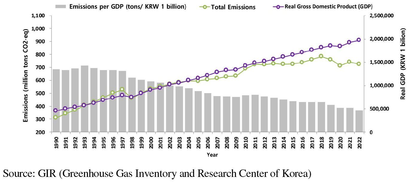
[Figure 1] illustrates the long-term trends in Korea’s environmental and economic performance from 1990 to 2022, revealing three dominant patterns: consistently exponential growth in real gross domestic product (GDP), a gradual inverse relationship in emission intensity (emissions per unit of GDP), and fluctuating yet persistently high total emissions. Real GDP has risen steadily over the past 30 years; in contrast, carbon emissions have declined only marginally in recent years. Significantly, emission intensity has decreased notably over the same period, reflecting a decoupling of emissions from economic growth; however, overall emissions remain high despite some increase in economic efficiency, indicating that South Korea has not yet achieved absolute decoupling. This situation underscores the need for a more robust, market-oriented climate policy, such as an ETS, to significantly reduce emissions in an economically efficient manner.
ETSs combine traditional regulatory enforcement with economic freedom, and are among the predominant market-based instruments for addressing climate change. Governments can set overall emissions targets and allow entities to sell emission allowances, thereby incentivizing reductions in emissions. Since the EU-ETS in 2005, ETSs have evolved from purely environmental policies into tools that influence energy and technological choices, as well as pathways and market performance.
Narassimhan et al. (2018) conducted a thorough comparison of implemented ETS systems worldwide, identifying divergence in market structure, design features, price stabilization instruments, allocation rules, and monitoring. Their analysis showed that policy efficiency depends greatly on system design elements, such as the stringency of the cap, the proportion of free allocation versus auctioning, and the inclusion or exclusion of market stability effectors. This situation indicates that ETS performance should be considered alongside institutional features and nuances in policy implementation, not just in terms of emissions reduction. The literature also underscores the importance of carbon price dynamics—including volatility, liquidity, and price discovery mechanisms—in determining how firms adjust to ETS policies. Exposure to stable carbon prices stimulates long-term investments in low-emission technologies; in contrast, excessive price volatility may lead to uncertainty, risk hedging by firms, and short-term compliance tactics. Consequently, carbon market performance is closely related to businesses’ costs and strategy choices, broadening the instrumentality of ETS from environmental regulation to an economic policy tool.
Policy evaluation research—particularly studies using DID frameworks—has been widely applied to estimate the causal effects of ETS implementation. For example, Yu et al. (2017) conducted a DID analysis to assess greenhouse gas reductions in South Korea before and after the introduction of the K-ETS, finding significant reductions in emissions attributable to the policy. Their results indicated that ETS could alter corporate behavior and drive emission reductions, while also revealing heterogeneity across industries and firm sizes.
Studies on K-ETS increasingly focus on environmental outcomes and economic and strategic implications. Unlike the EU-ETS, K-ETS initially featured high levels of free allocation and strong protection for energy-intensive and trade-exposed sectors. These structural differences imply that policy impacts may manifest differently in South Korea, potentially delaying market adjustments or altering corporate compliance strategies. Consequently, there is a growing need for research evaluating K-ETS from both environmental and financial perspectives. Accordingly, Khue et al. (2017) argued that the K-ETS significantly reduced carbon emissions of Korean companies while imposing some short-term financial burdens, but it did not have a significant negative impact in the mid to long term. In other words, environmental performance and financial performance can coexist rather than being a trade-off.
Fang and Chen (2017) confirmed that China’s human capital and energy consumption are major determinants of China's economic growth, and that human capital enhances its contribution to growth by improving energy use efficiency. Building on this, an expanded study Dechezleprêtre et al. (2022) examined China’s ETS pilot programs and found that ETS reduced emissions and improved firms’ financial performance and innovation outcomes. They emphasized that ETS should not be viewed solely as a regulatory burden; it is also an incentive mechanism that can stimulate technological progress and enhance corporate competitiveness. This finding aligns with the growing view that ETS has evolved into a policy-induced innovation driver.
At the firm level, previous studies have examined how ETS influences corporate responses through various channels, including compliance costs, energy-efficiency upgrades, R&D investment, green patenting, and strategic carbon management. Some firms initially face higher operational costs; however, long-term benefits often emerge through energy-saving technologies, improved reputation, and enhanced environmental, social, and governance (ESG) performance. Importantly, the size and impact of ETS effects vary between sectors, influenced by factors such as carbon intensity, costs of reduction, and ability to innovate.
Recent studies analyzing how climate change and carbon emission risks are reflected in stock returns from an asset pricing perspective have been accumulating. Bolton and Kacperczyk (2021) empirically examined the relationship between carbon emissions and stock returns for U.S. companies, suggesting that firms with higher emissions have higher expected returns. They interpret this as evidence of a risk premium, compensation for carbon-related risk. In other words, the market demands a higher required return by factoring in the possibility that companies with high emissions are more exposed to stricter regulations and transitional risks in the future. These discussions imply that environmental regulations do not solely affect corporate value directly by increasing or decreasing it; rather, they can influence asset prices through changes in corporate risk structures and adjustments in expected returns. The analysis in this study can also be linked to this asset pricing perspective, highlighting the need to consider that changes in returns observed after the implementation of the ETS system may result from risk premium adjustments as well as improvements in performance. Meanwhile, recent studies have examined whether the stock market can serve as an incentive to promote corporate decarbonization. According to Millischer et al. (2023), the stock market offers only limited rewards for reducing carbon emissions, making it difficult to achieve sufficient corporate decarbonization through market mechanisms alone. Consequently, the importance of policy regulation is increasingly emphasized.
Another recent research has shifted toward examining how ETS affects financial markets in Chapple et al. (2013), substantial valuation, stock returns, return volatility, and investor risk perception. ETS introduces carbon price signals that can serve as systematic risk factors, influencing firm valuation through expected future compliance costs and transition risks. Additional studies have found that carbon-intensive firms experience changes in stock price behavior after ETS implementation, suggesting that carbon exposure has become financially material (Park et al., 2024).
A closer examination of Park et al. (2024) reveals that the study reported a decline in Tobin’s Q for regulated companies following the introduction of the K-ETS. This decline was interpreted as reflecting negative market expectations regarding long-term corporate value. Simultaneously, the study found that the systematic risk (beta) of companies participating in the ETS had increased.
Park et al. (2024) focused their analysis on the first planning period; in contrast, this study aims to extend the analysis through the third planning period, after 2021. Additionally, this study seeks to verify whether the returns of companies participating in the ETS have increased, which could be interpreted as a risk premium associated with heightened risk. In other words, the market appears to be re-evaluating risk by incorporating uncertainties related to carbon prices and the potential for stricter future regulations. Accordingly, this study intends to confirm whether the expected rate of return has increased or decreased. Therefore, rather than contradicting the long-term decline in value reported by Park et al. (2024), this study can be understood complementarily from an asset pricing perspective, where increased risk corresponds with an increased expected rate of return.
Most prior studies have focused either on environmental outcomes or on corporate-level compliance behavior, without fully linking ETS to financial market responses. Furthermore, evidence from South Korea remains scarce, particularly regarding stock market reactions, corporate risk assessment, and firm heterogeneity in the context of ETS regulation; thus, a clear gap exists in the literature regarding how K-ETS influences capital markets and investor expectations.
This study aims to fill this gap by investigating how implementing the K-ETS affects stock returns of listed companies and whether the impact differs by industry, carbon intensity, and ESG characteristics. Using a DID-based econometric approach, we examine whether ETS functions merely as an environmental compliance mechanism or has evolved into a market-based policy that shapes firm valuation and investor behavior. This study’s findings provide novel insights into the financial relevance of ETS and contribute to the growing body of literature connecting climate policy, firm behavior, and capital markets.
Ⅲ. Data and Research Methodology
In this study, the analysis was conducted by dividing 100 listed companies into two groups in <Table 1>. 50 companies participating in the ETS and 50 companies not participating in the ETS. The limitation to 100 companies arises from the selection criteria applied to the ETS companies provided by GIR (Greenhouse Gas Inventory). Specifically, only companies with greenhouse gas emissions data from 2015 to 2023 were included. Additionally, explanatory variables such as profits, assets, debt ratio, and number of employees were simplified to include only companies with consistent data across the years. Since the research primarily focused on listed companies, the dependent variable was the stock price return of large and medium-sized firms. The exclusion of small and medium-sized enterprises (SMEs) represents a limitation of this study. However, efforts were made to select companies from various industries. ETS companies, which naturally emit greenhouse gases, were predominantly from the steel, chemical, and oil refining sectors, while non-ETS companies were mainly from the financial, pharmaceutical, and holding sectors (<Table B1>).
<Table 1>
Variables Used in the Empirical Analysis
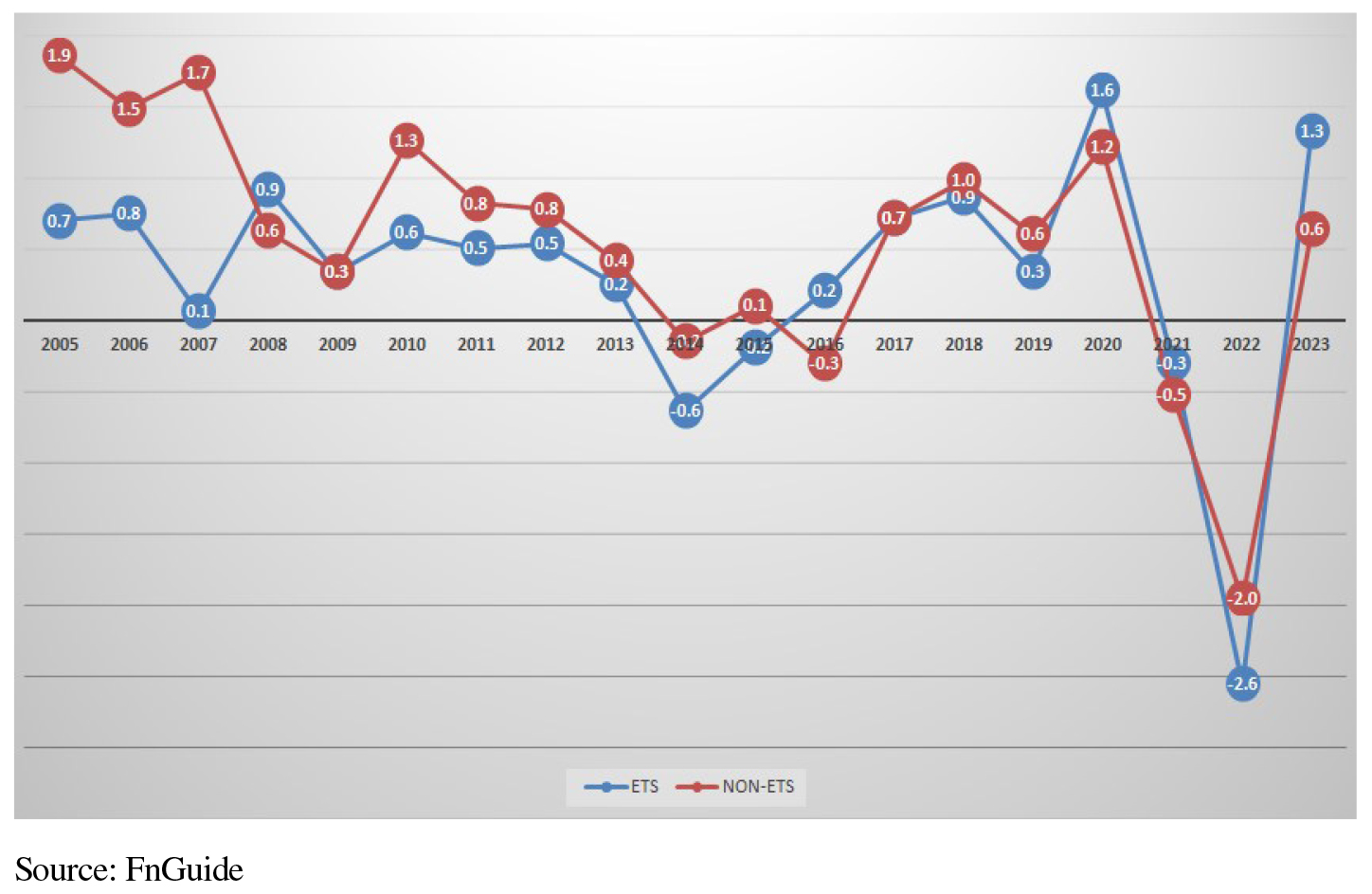
Like Oestreich and Tsiakas (2015) and Wen et al. (2020), the sample was divided into ETS target companies and non-target companies, and the difference in returns was analyzed. As shown in [Figure 2], ETS and non-ETS firms largely moved in parallel over the sample period, reflecting common macroeconomic shocks. The absence of a clear structural divergence immediately following the introduction of the ETS suggests that the system did not generate a significant direct cost shock. Instead, the estimated DID effects reflect relative adjustments within broadly similar return dynamics.
Our empirical analysis employs a comprehensive DID regression model1) to estimate the causal effect of ETS policy on firm-level stock returns. The expanded form of our baseline specification explicitly incorporates all control variables, fixed effects, and the treatment interaction term, providing a complete picture of our identification strategy. Equation (1) presents the complete regression.
Equation (1) represents our primary estimating relationship, where each component plays a specific role in isolating the treatment effect of interest while controlling for confounding factors and addressing various sources of bias.
The error term () represents idiosyncratic shocks to firm ’s stock return in year ; these shocks remain unexplained after accounting for treatment effects, control variables, and fixed effects. We impose a key constraint on the variance structure of these errors: . This specification acknowledges that error variances may differ across firms (heteroskedasticity) while allowing for arbitrary correlation of errors within the same firm over time. We implement this constraint using clustered standard errors at the firm level, yielding robust inference that accounts for both heteroskedasticity and within-firm serial correlation. Clustering at the firm level is conservative and appropriate, given that treatment varies across firms and errors are likely correlated within firms due to persistent unobserved shocks, measurement error, or other firm-specific factors.
The DID estimator provides an intuitive framework for interpreting our coefficient of interest (). Formally, the DID estimator can be expressed as follows:
This formulation highlights the two-stage comparison inherent in the DID design. The first term in parentheses () represents the average change in stock returns for treated firms (those subject to ETS) from the pre- to post-implementation periods. This “before-and-after” comparison for the treatment group captures the causal effect of ETS and any confounding time trends that would have occurred regardless of the policy.
The second term in parentheses () represents the analogous change for control firms (those not subject to ETS) over the same period. This comparison captures the counterfactual trend—how stock returns evolved for similar firms that did not experience the treatment. We can subtract the control group’s change from the treatment group’s change to effectively “difference out” common time trends, leaving an estimate of the pure policy effect.
The parallel trends assumption is the key identifying assumption underlying this interpretation: without ETS policy intervention, treatment and control firms would experience similar changes in stock returns over the study period. We do not observe the counterfactual; therefore, we cannot directly test this assumption for the posttreatment period. Nonetheless, it can be partially assessed by examining pre-treatment trends—the treatment and control groups following parallel trajectories before policy implementation would provide supporting evidence for this assumption.
The sign and magnitude of have important economic and policy implications. Three scenarios are possible, each corresponding to a different market assessment of ETS policy.
indicates a positive treatment effect. If the estimated coefficient is positive and significantly different from zero, the ETS policy increases stock returns for the treatment group relative to the control group. The positive effect suggests that the financial market is favorably evaluating the adaptability and potential competitiveness of companies subject to ETS regulation. This can be attributed to several factors, such as expectations for investment in low-carbon technologies, enhanced reputation, or increased awareness of expanding access to ESG-related capital. However, it is more appropriate to interpret these effects as reflections of market expectations or potential opportunities rather than as direct increases in corporate value.
Conversely, a negative, statistically significant indicates that the ETS policy decreases stock returns for the treatment group relative to the control group, suggesting that financial markets perceive ETSs as value-destroying or costly for regulated firms. This interpretation aligns with the traditional view that environmental regulations impose compliance costs, reduce operational flexibility, and constrain production possibilities. Such negative effects might arise from direct costs, such as purchasing emissions allowances, investing in abatement technologies, monitoring and reporting expenses, and administrative burdens. They could also reflect indirect costs, such as reduced competitiveness if rival firms in jurisdictions without carbon pricing gain cost advantages, stranded assets if carbon-intensive capital becomes obsolete, or heightened regulatory uncertainty that increases the cost of capital. A negative coefficient suggests that markets expect ETS compliance costs to exceed any potential benefits, thereby reducing profitability and growth opportunities and increasing risk for affected firms.
If the estimated coefficient is statistically indistinguishable from zero, stock returns experience no discernible policy effect. A null finding could emerge for several reasons. First, markets may have already incorporated expectations about ETS implementation into stock prices before the official policy announcement or during our pretreatment period. Such actions would lead to no additional price movement in the posttreatment period. Second, the costs and benefits of ETS may approximately offset each other, resulting in a net-zero impact on firm value. Third, ETS effects may be heterogeneous across firms, with some benefiting and others harmed, such that the average treatment effect masks important variation. Fourth, poorly designed or weakly enforced ETS policies, or those accompanied by extensive exemptions and free allowance allocations, may result in an effective treatment intensity insufficient to generate measurable stock market responses.
We extend our baseline DID specification to a multi-period framework to capture the evolving impact of ETS policy across distinct implementation phases. This extended model allows us to examine whether the ETS treatment effect on firm stock returns varies over time, reflecting potential learning effects, adjustment dynamics, policy refinements, or changing market perceptions as the regulatory regime matures. The multi-period specification is formalized in Equation (3).
Equation (3) generalizes our baseline model by partitioning the post-treatment period into multiple discrete phases, each with its own treatment effect coefficient. We estimate separate treatment effects across different periods to test hypotheses about the temporal evolution of policy impacts and to gain insights into the mechanisms through which ETS affects firm valuations.
represents the vector of lagged control variables and their corresponding coefficients (prime is transpose to multiply appropriately with matrices). As explained in the equation, it is a vector of lagged control variables: log profit, log assets, log debt, log employment, and salary. These are the five variables, all logarithmized and lagged by one period, proxying for prior differences in firm characteristics that may be related to both treatment status and performance.
The key innovation in this specification is the summation term, , which replaces the single interaction term from our baseline model. This summation structure allows us to estimate two separate treatment effect coefficients ( and ), corresponding to two distinct policy periods. The index ranges from 1 to 2, indicating that we partition our sample into three periods: a pre-treatment baseline period (before 2015) and two post-treatment phases.
The first treatment effect coefficient () captures the effect during the period from 2015 to 2020, which we interpret as the initial implementation phase of the ETS policy. This period represents the early years of carbon pricing, when firms and markets were first adjusting to the new regulatory environment. The interaction term equals one for treated firms (those subject to ETS) during the 2015-2020 window, and zero otherwise. Therefore, after accounting for contemporaneous changes in control firms and adjusting for all covariates and fixed effects, the coefficient measures the average change in stock returns for ETS firms during 2015-2020 relative to their pre-2015 baseline.
The interpretation of , as the “Effect during 2015-2020 (relative to pre-2015),” is crucial. This coefficient does not compare the 2015-2020 period to the 2021-2023 period. Instead, it compares the 2015-2020 outcomes for treated firms with what they would have been in the absence of treatment, using the pre-2015 period as the baseline and the control group to adjust for common trends. A positive indicates that ETS increased stock returns during this initial phase, perhaps because early compliance generated competitive advantages, improved corporate reputation, or signaled management quality to investors. Conversely, a negative suggests that the costs and uncertainties of early ETS implementation outweighed any benefits, depressing valuations for affected firms.
The second treatment effect coefficient () captures the effect during the period from 2021 to 2023, a later phase of ETS implementation with potentially different characteristics. The interaction term equals 1 for treated firms during the 2021-2023 window and 0 otherwise. The coefficient measures the average change in stock returns for ETS firms during 2021-2023 relative to their pre-2015 baseline, adjusting for control group trends and covariates.
The 2021-2023 period may differ from the 2015-2020 period in several important ways. By 2021, firms had several years of experience with ETS compliance, potentially reducing uncertainty and adjustment costs. Moreover, markets had observed actual outcomes rather than merely anticipating future impacts, possibly leading to more informed pricing. Additionally, the 2021-2023 period coincides with heightened global attention to climate change, increased investor focus on ESG factors, and, in many jurisdictions, strengthened climate policy ambitions, including net-zero commitments. The period may also reflect the implementation of policy changes that were “added on top of the existing ETS,” including stricter emissions caps, reduced free allowance allocations, expanded sectoral coverage, and enhanced enforcement mechanisms.
A key feature of this specification is that both and are estimated relative to the same pre-2015 baseline period; therefore, we can directly compare the two coefficients to assess whether treatment effects grew stronger, weaker, or remained stable over time. If (where the vertical bars denote absolute value), policy effects intensified in the later period. If , the effects diminished over time, possibly due to adaptation, learning, or diminishing marginal impacts. If , this would indicate relatively stable effects across the two phases.
Ⅳ. Regression Results
<Table 2>
Regression Results: ETS Policy Effects on Stock Returns
| Variable | Coefficient | (Std. Error) |
| Treatment Effect | ||
| 0.4993* | (0.2639) | |
| Lagged Controls | ||
| -0.0275 | (0.0503) | |
| -1.1289*** | (0.3470) | |
| 0.7140*** | (0.2340) | |
| -0.2277* | (0.1306) | |
| 0.0904*** | (0.0253) | |
| Firm Fixed Effects | Yes | |
| Year Fixed Effects | Yes | |
| Observations | 1,800 | |
| Number of Firms | 100 | |
| R-squared | 0.1968 | |
The regression in <Table 2> includes 1,800 observations across 100 firms, yielding a substantial panel dataset with adequate statistical power to detect economically meaningful treatment effects. The sample size implies an average of 18 observations per firm if the panel is balanced, though some firms may enter or exit at different times. The R-squared value of 0.1968 indicates that the model explains approximately 20% of the total variation in stock returns, which is quite respectable for stock return regressions, which are inherently noisy due to unpredictable factors, news shocks, and market dynamics that dominate short-term price movements. Our parsimonious model with treatment effects, five controls, and fixed effects captures nearly one-fifth of the return variation, suggesting the presence of meaningful systematic patterns; however, over 80% of the variation remains unexplained by observable factors. This outcome underscores both the inherent difficulty of predicting stock returns and the importance of using robust inference methods to account for this substantial residual uncertainty.
The parallel trends assumption is the key identification assumption of the DID model in [Figure 3]. The DID estimate can be interpreted as a causal effect only when this assumption holds; thus, its validity must be verified before presenting the results. The test examined whether the difference in trends between the treatment and control groups was statistically significant before policy implementation. Specifically, the model included interaction terms between time and treatment-group indicators at each pre-treatment time point to assess whether there is a systematic difference between the two groups before policy implementation. The test results were reported as an F-test for the null hypothesis so that the coefficients of the interaction terms for all seven pretreatment time points (from -8 to -2) were simultaneously 0. The test yielded F(7, 99) = 1.29, p = 0.2643, indicating that the null hypothesis cannot be rejected at the 5% significance level. This result indicates that, prior to the policy implementation, the trends in the treatment and control groups do not differ in a statistically significant way. These test results provide a crucial foundation for validating the DID model. The p-value is 0.2643, which is significantly greater than the 0.05 significance level; therefore, we can conclude that the parallel trends assumption—that the treatment and control groups exhibited similar trends before the policy implementation—is satisfied.
This outcome implies that the observed difference between the two groups after the policy implementation meets essential prerequisites for being interpreted as a causal effect of the policy. If the null hypothesis had been rejected in the pretrend test, it would indicate that the two groups followed different trends before the policy, making it difficult to interpret the post-policy difference as a pure policy effect; therefore, the results of this test suggest that the DID identification strategy employed in this study is appropriate, and the causal interpretation of the estimated policy effect is valid. Nonetheless, this test only examines observable trends; thus, additional robustness checks may be necessary to account for unobserved factors. Consequently, further robustness tests will be conducted later.
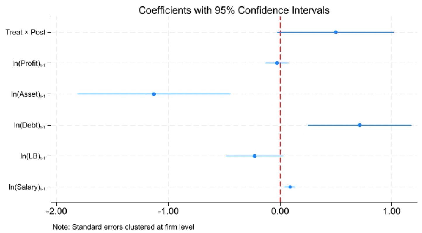
<Table 2> presents our main regression results examining the causal effect of ETS policy implementation on firm-level stock returns using a DID framework. The coefficient of primary interest is the treatment effect, captured by the interaction term . This term measures the differential change in stock returns for ETS-regulated firms during the post-implementation period. The estimated coefficient is 0.4993 with a clustered standard error of 0.2639, statistically significant at the 10% level (p < 0.10), suggesting that ETS policy increases stock returns for treated firms by approximately 0.50 percentage points on average, holding all else constant.
The positive coefficient does not necessarily indicate that the emissions trading system increased firm value. Instead, this result may reflect adjustments in expected returns associated with the transition to a carbon-constrained economy. Specifically, financial markets may demand higher returns from firms exposed to potential regulatory or transition risks related to carbon emissions. The estimated treatment effect of approximately 0.50 percentage points should therefore be interpreted with caution. Rather than indicating that the ETS directly improved firm performance, the positive return differential may reflect changes in investors’ required returns for firms exposed to carbon-related transition risks. This interpretation aligns with recent literature suggesting that carbon exposure can influence expected returns through a carbon risk premium.
When compounded over time and across market capitalizations, a half-percentage- point boost to annual returns indicates substantial cumulative shareholder value. From a policy perspective, these findings suggest that financial markets are beginning to incorporate carbon-related transition risks into asset prices. As carbon pricing policies become more stringent and carbon prices increase over time, these risks are likely to be reflected more prominently in financial markets.
The regression includes five lagged control variables capturing key firm financial characteristics. The coefficient on is -1.1289 (SE = 0.3470) and highly significant at the 1% level, indicating that larger firms tend to experience considerably lower subsequent stock returns. This negative relationship aligns with the well-documented size effect in asset pricing, where smaller firms often exhibit higher average returns due to greater risk, lower liquidity, or higher growth opportunities. The magnitude of -1.13 suggests that a 1% increase in lagged assets is associated with approximately a 1.13 percentage-point decrease in returns, representing a substantial effect that underscores the importance of controlling for firm size.
The coefficient on is 0.7140 (SE = 0.2340) and highly significant at the 1% level, indicating that more leveraged firms experience higher stock returns. This positive relationship may reflect leverage amplifying equity returns, management confidence signaled by debt financing, or advantageous borrowing conditions that enable firms to exploit investment opportunities. These two highly significant controls—assets and debt—demonstrate that firm size and capital structure are crucial predictors of equity performance and must be accounted for to isolate the ETS treatment effect.
The coefficient on is -0.0275 (SE=0.0503) and statistically insignificant at conventional levels, suggesting that year-to-year fluctuations in profit (beyond what firm and year fixed effects capture) do not strongly predict subsequent returns in our specification.
The coefficient on is -0.2277 (SE=0.1306) and marginally significant at the 10% level, indicating that firms with higher book values tend to experience modestly lower returns, potentially reflecting value-growth dynamics.
Most notably, the coefficient on is 0.0904 (SE = 0.0253) and highly significant at the 1% level, indicating that firms with higher salary expenditures experience higher subsequent returns. This relationship could reflect factors particularly relevant for understanding ETS compliance capabilities, such as higher-quality human capital, greater innovation capacity, or skilled workforces better positioned to adapt to regulatory changes. Collectively, these controls absorb substantial variation in outcomes. The highly significant effects on assets, debt, and salary demonstrate that firm financial characteristics meaningfully predict stock returns, even after controlling for fixed effects, thereby increasing the precision of estimating the treatment effect of interest.
<Table 3>
Multiperiod DID Estimates: ETS Policy Effects on Stock Returns
| Variable | Coefficient | (Std. Error) | t |
| Treatment Effect | |||
| 0.4963* | (0.2858) | 1.74 | |
| 0.5052 | (0.3299) | 1.13 | |
| Lagged Controls | |||
| -0.0274 | (0.0504) | -0.54 | |
| -1.1287*** | (0.3446) | -3.28 | |
| 0.7139** | (0.2333) | 3.06 | |
| -0.2277** | (0.1306) | -1.74 | |
| 0.0905*** | (0.0255) | 3.54 | |
| Firm Fixed Effects | Yes | ||
| Year Fixed Effects | Yes | ||
| Observations | 1,800 | ||
| Number of Firms | 100 | ||
| R-squared | 0.1968 | ||
<Table 3> presents our extended DID regression results that decompose ETS policy effects across two distinct implementation phases: Period 1 (2015-2020) and Period 2 (2021-2023). Both periods are measured relative to the pre-2015 baseline. This specification allows us to examine whether treatment effects evolve as firms adapt to regulations, markets incorporate new information, and policies are refined. The model estimates two separate treatment effects. The coefficient on captures the effect during the initial 2015-2020 implementation phase. The captures the effect during the later 2021-2023 phase (when the scheme was already established and additional policy changes had been implemented). By estimating period-specific coefficients, we can assess whether ETS impacts strengthen, weaken, or remain stable as the regulatory regime matures. This approach provides insights into learning effects, adjustment dynamics, and the incremental impact of policy modifications layered onto the existing framework in [Figure 4].
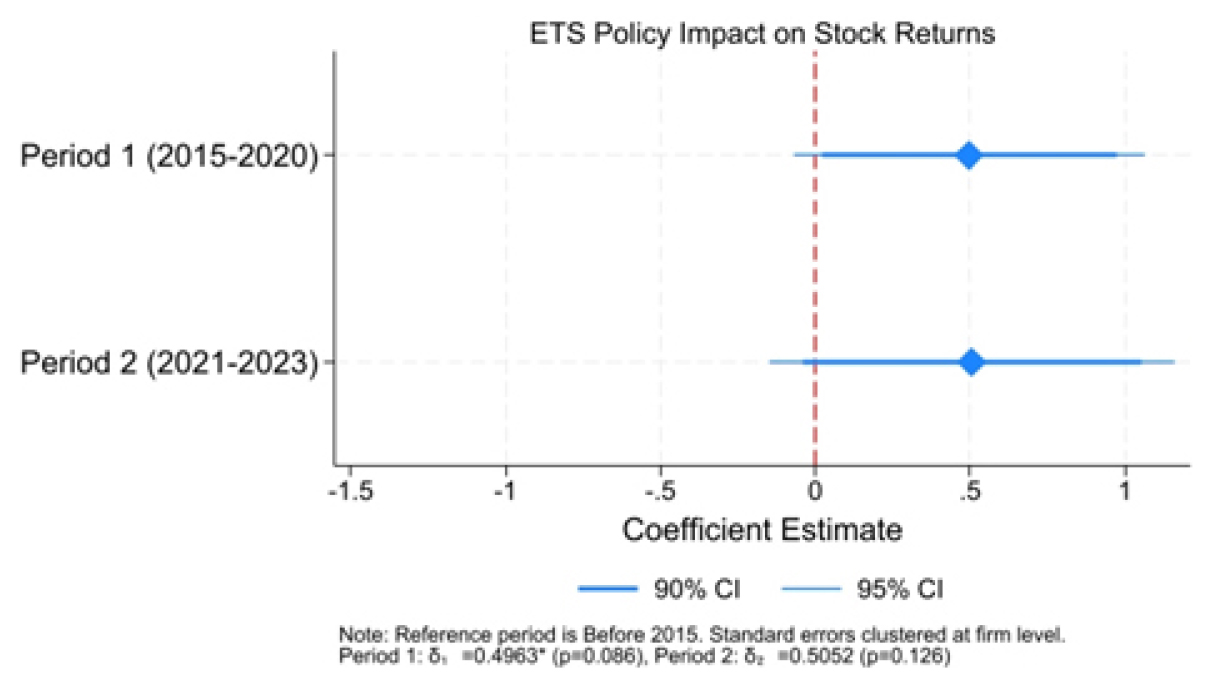
The coefficient on Treat × Period 1 (2015-2020) is 0.4963, with a standard error of 0.2858, yielding a t-statistic of 1.74 and a p-value of 0.086. This estimate is statistically significant at the 10% level, indicated by a single asterisk. After controlling for contemporaneous changes in control firms and adjusting for firm characteristics and fixed effects, the positive coefficient suggests that during the initial implementation phase from 2015 to 2020, ETS policy increased stock returns for treated firms by approximately 0.50 percentage points relative to the pre-2015 baseline. This finding indicates that financial markets viewed the initial implementation of the ETS favorably, with benefits apparently outweighing compliance costs. The observed positive return differential may also reflect investors’ reassessment of regulatory risks following the introduction of the ETS. Rather than indicating direct economic benefits, this effect may capture adjustments in risk perceptions related to carbon regulation and future climate policies.
The coefficient on Treat × Period 2 (2021-2023) is 0.5052, with a standard error of 0.3299, yielding a t-statistic of 1.13 and a p-value of 0.129. This estimate is not statistically significant at conventional levels, falling short of even the 10% threshold. The point estimate of approximately 0.51 percentage points is remarkably similar in magnitude to the Period 1 effect, suggesting that the average treatment effect remained relatively stable across the two phases. In contrast, the larger standard error (0.33 versus 0.29) and resulting loss of statistical significance indicate greater uncertainty in the later period. This result may be due to a smaller sample size (fewer years in Period 2), increased volatility in stock returns, or more heterogeneous responses across firms as the policy environment became more complex. Interpreting this coefficient requires careful attention to the institutional context. Period 2 represents a phase when “the scheme was already established, and the price rule changes were added on top of the existing ETS,” meaning we are estimating the effect of incremental policy modifications rather than the initial introduction of carbon pricing. The similarity between and (0.50 versus 0.51, respectively) suggests that the marginal effect of these later policy changes was approximately equal to the original ETS effect; however, insufficient statistical significance precludes strong conclusions about whether the later modifications meaningfully altered firm valuations.
The lagged control variables show patterns largely consistent with our baseline results. The coefficient on is -0.0274 (SE = 0.0504) and statistically insignificant (p = 0.588), indicating that year-to-year profit fluctuations (beyond what fixed effects capture) do not strongly predict returns. The coefficient on is -1.1287 (SE = 0.3446) and highly significant at the 1% level (p = 0.001), confirming the strong negative relationship between firm size and subsequent returns consistent with the size effect in asset pricing. The coefficient on is 0.7139 (SE = 0.2333) and highly significant (p = 0.003), maintaining the positive leverage-return relationship observed in our baseline specification. Interestingly, the coefficient on is -0.2277 (SE = 0.1306) and marginally significant (p = 0.084), showing a negative association between book value and returns. The coefficient on is 0.0905 (SE = 0.0255) and highly significant (p = 0.001), confirming that firms with higher salary expenditures experience better stock performance, likely reflecting human capital quality or operational sophistication. These remarkably stable control-variable coefficients across specifications provide reassurance that our results are robust and that the multi-period decomposition does not materially alter the underlying relationships between firm characteristics and returns, thereby strengthening confidence in our modeling approach.
[Figure 5] presents the results of an event study analyzing how ETS policy implementation affects stock returns over time. The X-axis represents the relative time, spanning 8 periods before and after the ETS policy implementation (denoted as 0); the Y-axis measures the effect on stock returns. The blue dots show the estimated values at each time point, while the vertical lines depict the 95% confidence intervals, visually illustrating the level of uncertainty in the estimates. The red dotted line at 0 serves as a baseline, distinguishing between positive and negative effects. Examining the period before the event (-8 to -1), the yield effect fluctuates around 0, suggesting no systematic change in returns before the ETS policy implementation. The lowest value is -0.99, and the highest is 0.92; this volatility falls within the range of normal market fluctuations.
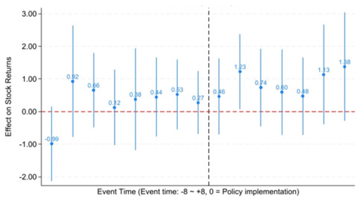
A positive effect of 0.27 is observed at the time of ETS policy implementation (period 0). In the subsequent periods (+1 to +8), the overall positive return effect continues and gradually increases. Notably, the effect peaks at 1.13 during period +6 and remains high at 1.88 in period +7, suggesting that the positive impact on stock returns reaches its maximum approximately 6 to 7 periods after the policy implementation. Conversely, as time progresses, the confidence interval widens, indicating increased uncertainty in the estimates. Additionally, since the confidence interval includes zero at most points, it is difficult to conclude that an effect is statistically significant except at specific points. Overall, these results suggest that the introduction of the ETS is associated with changes in the relative stock returns of regulated versus non-regulated companies. However, these patterns may reflect risk-pricing dynamics rather than improvements in corporate performance or value, and therefore should be interpreted with caution.
The baseline model in this study addressed issues of simultaneity and reverse causality by applying a one-period lag to the control variables. However, in the case of the K-ETS, there may be institutional time lags between the corporate designation date (e.g., 2014), the system implementation date (2015), and the realization of costs through emission reporting and settlement (e.g., 2016). The event study figure also shows that the effect becomes more apparent 1-2 years after the policy introduction rather than immediately. Considering these factors, it is necessary to examine the possibility that the policy effect is reflected in the market with a certain time lag rather than instantaneously in the rate of return.
Accordingly, this study conducted an additional analysis using a one-year lead for the dependent variable. In other words, it tested whether the institutional change at the time of policy implementation was reflected in the following year’s rate of return. The estimation results showed that the positive effect on the returns of ETS target companies remained consistent with the baseline model, with statistical significance confirmed at the 10% level. This suggests that the policy effect is not a short-term event response but rather reflects the market’s gradual adjustment of expectations regarding institutional changes over time. These findings indicate that the main conclusions of this study are not driven by short-term fluctuations in any specific year but are based on changes in relative returns observed after policy implementation.
<Table 4>
Multiperiod DID Estimates: Robustness Check 1 (Period = 2 if the Year 2022)
| Variable | Coefficient | (Std. Error) | t |
| Treatment Effect | |||
| 0.5154* | (0.2744) | 1.88 | |
| 0.4431 | (0.4049) | 1.09 | |
| Lagged Controls | |||
| -0.0279 | (0.0505) | -0.55 | |
| -1.1301*** | (0.3446) | -3.28 | |
| 0.7146*** | (0.2327) | 3.07 | |
| -0.2281* | (0.1305) | -1.75 | |
| 0.0901*** | (0.0255) | 3.53 | |
| Firm Fixed Effects | Yes | ||
| Year Fixed Effects | Yes | ||
| Observations | 1,800 | ||
| Number of Firms | 100 | ||
| R-squared | 0.1969 | ||
<Table 5>
Multiperiod DID Estimates: Robustness Check 2 (Drop 2021)
| Variable | Coefficient | (Std. Error) | t |
| Treatment Effect | |||
| 0.8928 | (0.5748) | 1.55 | |
| Lagged Controls | |||
| -0.0035 | (0.0543) | -0.07 | |
| -1.2356*** | (0.4156) | -2.97 | |
| 0.7473** | (0.2918) | 2.56 | |
| -0.2232* | (0.1329) | -1.68 | |
| 0.0974*** | (0.0257) | 3.78 | |
| Firm Fixed Effects | Yes | ||
| Year Fixed Effects | Yes | ||
| Observations | 1,600 | ||
| Number of Firms | 100 | ||
| R-squared | 0.1246 | ||
<Table 4> and <Table 5> present two robustness checks that test the sensitivity of our main findings against alternative temporal definitions and sample compositions. These robustness analyses establish the credibility and generalizability of our core results by assessing whether treatment effect estimates depend critically on specific modeling choices or remain stable across reasonable alternative specifications. <Table 4> implements robustness check 1, which redefines Period 2 to include only 2022-2023 rather than 2021-2023, treating 2021 as a transition year and focusing on the most recent years when policy changes were fully implemented. <Table 5> implements robustness check 2, which excludes 2021 entirely from the analysis and estimates a simpler two-period model with just . This approach effectively collapses back to the baseline specification but with a truncated sample. Comparing results across these alternative specifications enables us to assess whether our findings are robust to reasonable variations in how we partition periods and define the post-treatment era, or whether they are artifacts of particular temporal boundaries that coincide with idiosyncratic shocks or structural breaks unrelated to ETS policy.
<Table 4> presents results in which Period 2 is redefined to include only 2022-2023 (rather than 2021-2023), resulting in a narrower two-year window. The coefficient on Treat × Period 1 (2015-2021) is 0.5154 with a standard error of 0.2744, yielding a t-statistic of 1.88 and p-value of 0.063, achieving marginal significance at the 10% level (indicated by a single asterisk). This estimate of approximately 0.52 percentage points is highly similar to our Period 1 coefficient of 0.50 in the main specification, indicating that the initial implementation-phase effect is robust to minor adjustments in the period boundaries. The coefficient on Treat × Period 2 (2022-2023) is 0.4431 with a standard error of 0.4049, yielding a t-statistic of 1.09 and a p-value of 0.276, which is not statistically significant at any conventional level. The point estimate of 0.44 percentage points suggests a positive effect slightly smaller than in Period 1, though the large standard error (0.40) reflects substantial uncertainty. The lack of significance is unsurprising given that Period 2 now spans only two years (2022-2023), severely limiting sample size and statistical power. Notably, even when narrowing the definition to focus exclusively on the most recent years when policy refinements should be most evident, the point estimate remains positive and of similar magnitude to Period 1, suggesting temporal stability; however, the doubled standard error relative to Period 1 (0.40 versus 0.27) indicates that precision declines intensely when estimating effects over such a short window, creating difficulties when concluding whether late-period modifications had distinct effects.
Comparing <Table 4> with our main <Table 3> results reveals important insights about sensitivity to period definitions. In <Table 3>, Period 1 (2015-2020) had a coefficient of 0.4963 (p = 0.086), while in <Table 4>, extending Period 1 through 2021 yields a coefficient of 0.5154 (p = 0.063), representing a modest increase in both magnitude and statistical significance. These findings suggest that including 2021 in the earlier period slightly strengthens the estimated effect, possibly because 2021 exhibited particularly favorable outcomes for ETS firms or because the longer time window increases statistical power. Conversely, the Period 2 coefficients decline from 0.5052 (p = 0.129) in <Table 3> (covering 2021-2023) to 0.4431 (p = 0.276) in <Table 4> (covering only 2022-2023), showing both a smaller point estimate and much weaker significance. The substantial increase in the standard error from 0.33 to 0.40, despite a similar point estimate, indicates that the precision loss from dropping one year of data outweighs any potential benefit from focusing on a more homogeneous post-modification period. The overall pattern—positive coefficients of similar magnitude (0.44-0.52) across all period definitions, though varying in statistical significance—supports the interpretation that ETS effects are relatively stable over time and positive on average; however, estimates are noisy, and precision depends heavily on sample size. These results do not change dramatically when we shift the Period 1/Period 2 boundary from 2020 to 2021, which provides evidence against our findings being artifacts of arbitrary cutoff dates coinciding with unrelated structural breaks.
The control variable coefficients in <Table 4> remain highly consistent with previous specifications, further supporting robustness. The coefficient on is -0.0279 (SE = 0.0505, p = 0.581). The coefficient on is -1.1301 (SE = 0.3446, p = 0.001), almost identical to <Table 3>’s -1.1287, maintaining strong significance at the 1% level and confirming the robust negative size effect. The coefficient on is 0.7146 (SE = 0.2327, p = 0.003), nearly identical to <Table 3>’s 0.7139, preserving the strong positive leverage effect at the 1% significance level. The coefficient on is -0.2281 (SE = 0.1305, p = 0.084), essentially unchanged from <Table 3> (-0.2277), maintaining marginal significance at the 10% level. The coefficient on is 0.0901 (SE = 0.0255, p = 0.001), trivially different from <Table 3> (0.0905), preserving strong significance at the 1% level. This remarkable stability of control variable coefficients across specifications—with point estimates changing by less than 1% and significance levels remaining constant—provides strong evidence that our modeling approach is sound. Moreover, the relationships between firm characteristics and returns are robust to temporal partitioning choices, and the treatment effect estimates are not driven by misspecification of the control structure. The R2 of 0.1969 in <Table 4> is virtually identical to <Table 3> (0.1968), confirming that redefining period boundaries does not materially alter overall model fit or explanatory power.
<Table 5> demonstrates an alternative robustness check that excludes 2021 from the sample and reverts to a simpler baseline specification with a single interaction rather than separate period effects. This approach treats 2021 as a potentially troublesome transition year that could distort estimates due to exceptional circumstances (e.g., post-pandemic recovery dynamics, policy uncertainty across time periods, or idiosyncratic shocks), and it assesses the impact when these are omitted. The sample size is reduced by 200 observations. The coefficient on is 0.8928 with a standard error of 0.5748, yielding a t-statistic of 1.55 and p-value of 0.124, which is not statistically significant at conventional levels. The point estimate of approximately 0.89 percentage points is substantially larger than the coefficients in <Table 2>, <Table 3>, <Table 4>, suggesting that when 2021 is excluded, the average treatment effect across the remaining post-2015 years appears more positive. However, the large standard error (0.57 v. 0.26-0.40 in the previous table) leads to greater uncertainty, and we lose statistical significance; therefore, we can say with much less confidence that the coefficient is different from zero here anyway. More variation may be due to a smaller sample size, greater heterogeneity in outcomes (if 2021 is firmly dropped), and instability in the oversimplified model, which, while clearly distinguishing pre-treatment from post-treatment phases, is included in this latter model regardless of the number of them.
Comparing model fit statistics across tables provides insights into specification performance. <Table 3> and <Table 4> both use 1,800 observations across 100 firms with multi-period frameworks. They achieve R2 values of 0.1968 and 0.1969, respectively. These results are nearly identical, suggesting that alternative period boundary definitions do not materially affect explanatory power when full samples are used. In contrast, <Table 5>, with 1,600 observations (excluding 2021) and a simplified single-period model, shows an R2 of 0.1246, representing a substantial 37% reduction in explained variation relative to <Table 3>, <Table 4>. This decline suggests that excluding 2021 and collapsing temporal heterogeneity into a single treatment effect both reduce the model’s ability to fit the data. The lower R2 could reflect loss of information from excluding 100 observations, loss of explanatory power from not distinguishing between different posttreatment phases (with potentially different effect sizes), or increased residual variance (if 2021 contained important systematic patterns that the remaining years cannot fully capture). All three tables include identical fixed-effect structures (firm and year FE) and control variables, suggesting that differences in R2 stem primarily from sample composition and temporal modeling choices rather than from fundamental specification differences. The consistency of R2 across <Table 3>, <Table 4> despite shifting period boundaries provides evidence that our multi-period approach is robust and not overfitting to idiosyncratic features of particular year groupings.
Synthesizing across both robustness checks yields several key conclusions about our main findings. First, the treatment effect point estimates are consistently positive across all specifications, ranging from 0.44 to 0.89 percentage points, with most estimates clustering around 0.44-0.52. This consistency in sign and approximate magnitude provides strong evidence that ETS policy is associated with positive effects on stock returns, regardless of specific modeling choices; however, the exact size remains somewhat uncertain. Second, statistical significance varies across specifications: Period 1 effects typically reach marginal significance (p = 0.063-0.086), whereas Period 2 and alternative specifications often fall short of conventional thresholds. This pattern suggests that treatment effects are detectable with an adequate sample size and appropriate temporal modeling but are not overwhelmingly large relative to noise in stock returns; thus, they require careful analysis to identify. Third, control variable coefficients are remarkably stable across <Table 2>, <Table 3>, <Table 4>, with point estimates changing by less than 2% and significance patterns unchanged. Nonetheless, they show more variation in <Table 5> when the sample size is reduced, indicating that the multi-period specifications with full samples provide more reliable parameter estimates across the board. Fourth, the larger but insignificant coefficient in <Table 5> (0.89, p = 0.124) compared to other specifications (0.44-0.52, p = 0.063-0.276) illustrates the precision-magnitude tradeoff. Excluding 2021 yields a larger point estimate; however, the increased standard error and loss of significance mean we have less confidence in this larger effect, suggesting that including all available data and modeling temporal heterogeneity explicitly is preferable for robust inference.
This study presents results from a DID model, showing that the stock price returns of ETS target companies have increased on average compared to non-target companies since the introduction of K-ETS. However, an analysis focusing solely on changes in average returns makes it difficult to determine whether the observed increase reflects a value gain due to improved corporate cash flows or compensation for increased risk. Therefore, the DID analysis was extended to include cash flow and profitability indicators, along with risk proxies (the absolute value and square of returns) available in the annual data, to distinguish whether the return increase was driven by enhanced value (improved cash flow) or risk compensation.
By analyzing the absolute and squared values of returns as proxy variables for risk using annual data, it was found that the absolute rate of return for processing companies increased significantly during the early stages of ETS introduction (2015 to March 2021), indicating a potential rise in risk. This pattern suggests that some of the increase in average yields may be related to risk premiums associated with carbon conversion exposure. However, after April 2021, the risk proxy variable is no longer statistically significant, making it difficult to attribute subsequent yield differences solely to risk compensation. One possible interpretation is that, as the ETS becomes more established, market uncertainty surrounding the policy has gradually diminished, reducing the extent to which conversion risk is reflected in expected returns. DID analysis of operating margin does not reveal a statistically significant change, making it difficult to interpret an increase in return as an improvement in cash flow. Similarly, the insignificance of the risk proxy after 2021 suggests that the return differences observed in the later period are unlikely to be explained solely by risk compensation. Instead, these differences may reflect changes in market expectations as the ETS institutional framework became more predictable and policy uncertainty declined (see <Table B2>).
In addition, to further validate the results of this empirical analysis, the interaction term between carbon intensity and carbon price for ETS companies was examined. Using GIR data, carbon intensity was calculated based on the annual carbon emissions and sales of ETS companies, while the monthly carbon price was averaged annually to determine the yearly carbon price. The positive interaction between changes in carbon prices and firm-level carbon intensity indicates that firms with greater carbon exposure tend to experience stronger stock return responses when carbon prices rise. This finding suggests that financial markets react to carbon pricing signals, particularly for firms with higher transition exposure. Therefore, the DID estimates in this study are more likely to capture changes in regulatory expectations associated with the implementation of the ETS rather than the direct cost effects of carbon prices themselves (see <Table B3>).
Ⅴ. Conclusion
Although the Korean ETS is characterized by a high proportion of free allocation and limited cost pass-through, these institutional features suggest that the direct cost impact on enterprises during the sample period may have been relatively minimal. Therefore, the observed stock return response is more likely related to perceived diversion risk or changes in regulatory expectations rather than immediate cost pressures. In fact, a limited immediate cost burden combined with increased regulatory clarity may generate a market revaluation effect rather than a pure cost shock. Therefore, our estimates should be interpreted as capturing the relative stock market revaluation associated with ETS participation under Korea’s institutional framework, rather than the direct causal impact of carbon prices on firm cash flows. Although concurrent ESG-related policy developments may have influenced firm valuations during the sample period, the inclusion of year fixed effects helps mitigate common macro-level shocks. Our empirical analysis examining the effect of the ETS policy on firm stock returns yields consistently positive, though modest and marginally significant, treatment effects across multiple specifications. The baseline DID model (<Table 3>) estimates that ETS implementation increases stock returns for treated firms by approximately 0.50 percentage points (β = 0.4993, p = 0.061), significant at the 10% level. The multiperiod specification (<Table 4>) decomposes this effect over time, revealing remarkable stability across implementation phases: Period 1 (2015-2020) shows a coefficient of 0.4963 (p = 0.086), and Period 2 (2021-2023) yields a coefficient of 0.5052 (p = 0.129), with nearly identical magnitudes. However, Period 2 loses statistical significance due to larger standard errors from the shorter time window. Robustness checks that redefine period boundaries (<Table 4>: Period 2 as 2022-2023 only) or drop 2021 entirely (<Table 5>: simplified specification with 1,600 observations) yield treatment effects ranging from 0.44 to 0.89 percentage points, all positive but varying in precision. The consistently positive signs across alternative model specifications should therefore be interpreted with caution. Rather than indicating that financial markets viewed the ETS as value-enhancing, the results are consistent with the possibility that investors adjusted expected returns to account for carbon-related transition risks and regulatory uncertainty. In this interpretation, higher observed returns may reflect compensation for exposure to such risks rather than improvements in firm performance.
Furthermore, firm financial characteristics consistently and significantly predict stock returns across all specifications, with remarkably stable coefficients that strengthen confidence in our modeling approach. Firm size, measured by , exhibits a strong negative relationship with returns; coefficients range from -1.13 to -1.24 and are consistently significant at the 1% level. These results are consistent with the well-documented size effect in asset pricing, in which smaller firms exhibit higher average returns. Moreover, financial leverage, measured by , shows a robust positive relationship (coefficients around 0.71-0.75, significant at 1%-5% levels). These results indicate that more leveraged firms experience higher equity returns, possibly reflecting leverage amplification effects or positive signals from debt financing capacity. Additionally, labor costs, measured by , demonstrate strong positive effects (coefficients around 0.09-0.10, highly significant at 1% level), suggesting that firms with higher salary expenditures—potentially proxying for human capital quality or operational sophistication—achieve better stock performance. In contrast, lagged profitability shows no significant relationship with returns (coefficients near 0, and p-values > 0.58), while the labor value exhibits modest negative effects (coefficients around -0.22 to -0.23, marginally significant at 10% level). These control-variable patterns remain virtually unchanged across <Table 3>, <Table 4>, <Table 5> despite different temporal specifications, with coefficients varying by less than 2%, providing strong evidence against model misspecification and supporting the interpretation that our treatment effect estimates are not artifacts of omitted-variable bias or confounding by firm characteristics.
The multiperiod and robustness analyses reveal important insights about temporal evolution and specification sensitivity. The near-identical treatment effects in Periods 1 (2015-2020) and 2 (2021-2023) of approximately 0.50 percentage points suggest remarkable stability in market assessments of ETS over time. Moreover, this stability indicates no strengthening effects from learning and adaptation or weakening effects from escalating costs or policy fatigue. This stability persists even when Period 2 includes only 2022-2023 (<Table 4>); however, statistical significance weakens due to the shorter sample periods. Excluding 2021 and reverting to a simplified specification (<Table 5>) produces a larger point estimate of 0.89, with doubled standard errors and loss of significance. This change illustrates the precision-magnitude tradeoff and suggests that multi-period frameworks utilizing full samples provide more reliable inference than simplified models with truncated data. Model fit statistics support this interpretation. R2 values of 0.1968-0.1969 across multi-period specifications with 1,800 observations indicate stable explanatory power. At the same time, dropping to 0.1246 in the simplified 1,600-observation model suggests information loss from excluding data and from collapsing temporal heterogeneity. The positive treatment effects are consistent (ranging from 0.44 to 0.52 percentage points) across <Table 3>, <Table 4>, <Table 5>, and the control variable estimates are robust; therefore, our findings are not artifacts of arbitrary modeling choices or overfitting to idiosyncratic features of particular year groupings.
Therefore, the positive treatment effects observed in this study should not be interpreted as evidence that environmental regulations enhance corporate value. Instead, the results suggest that the introduction of ETS may be associated with adjustments in expected returns for companies exposed to carbon-related transition risks. In this context, these findings align with emerging literature (Bolton and Kacperczyk, 2021) on carbon risk premiums, which posits that investors demand higher returns from companies more vulnerable to climate policy risks. Although the estimated effect is minimal and only statistically significant to a limited extent, it indicates that financial markets may begin incorporating carbon transition risks into asset prices, even in a regulatory environment where carbon prices remain relatively low. As carbon pricing policies become more stringent and transition risks escalate, these dynamics are likely to become more pronounced. ETS effects are not overwhelmingly positive, and substantial uncertainty remains about the exact magnitudes. The strong and stable effects of firm size, leverage, and labor costs on returns suggest that ETS impacts likely vary systematically across firm types. Such variation implies that differentiated policy provisions or targeted assistance programs could enhance both efficiency and equity. For researchers, our study demonstrates the value of comprehensive robustness checking and of multiperiod frameworks that explicitly model temporal dynamics. Moreover, conservative inference using clustered standard errors and multiple specifications is essential for establishing that the findings are not fragile artifacts of specific assumptions. Future research should extend these analyses with longer posttreatment samples as data accumulate. Additionally, studies can explore heterogeneous effects across firm characteristics and industries, examine alternative outcome measures beyond stock returns to assess real economic impacts, and conduct comparative studies across multiple ETS implementations to identify design features that maximize environmental effectiveness while minimizing economic disruption.
