

Ⅰ. Introduction
Ⅱ. Literature Review
Ⅲ. Data and Variables
Ⅳ. Estimation models
Ⅴ. Estimation Results
Ⅵ. Summary and Policy Implication.
Ⅰ. Introduction
Climate change is affecting lives, livelihoods, health, food and water security, infrastructure, and environments around the world. One of the main causes of climate change is the burning of fossil fuels, including oil, natural gas and coal which account for over 75 per cent of global greenhouse gas (GHG) emissions and about 90 per cent of total carbon dioxide emissions. The Korean government has been actively engaged in efforts to tackle climate change and believes that such actions provide opportunities to create future drivers of economic growth. In 2009, the Korean government announced that it would reduce GHG emissions by 30% from their business-as-usual (BAU) level by 2020.
In June 2015, Korea submitted a Nationally Determined Contribution (NDC) target to the Secretary of the The Intergovernmental Panel on Climate Change (IPCC). The target stated that by 2030, Korea planned to reduce its greenhouse gas (GHG) emissions by 37% from the Business-As-Usual (BAU) level. In 2021, Korea updated its NDC target for 2030, committing to a 40% reduction in GHG emissions compared to the levels recorded in 2018. To achieve 2030 NDC target, Korean government has committed to gradually phasing out coal-fired power generation and expanding the share of renewable energy. The third Energy Master Plan (MOTIE, 2019) set a new and more ambitious goal of increasing the share of renewable electricity to 20% by 2030, and to 30-35% by 2040. Expansion of renewable energy sector is expected to contribute to mitigating climate change and enhancing energy security. In 2020, South Korea has invested about 42 trillion KRW ($36.6 billion) in the renewable energy sector to meet the annual production of 13 million kilowatts of electricity, equivalent to 26 coal power plants. As predicted in the Renewable Energy 3020 Plan, solar and wind power capacity will reach 36.5GW and 17.7GW respectively by 2030.
Over the last decade, the Levelized Cost of Energy (LCOE) of renewable energy has declined rapidly (Anon, 2019), but it is still higher than the LCOE of conventional energy sources such as coal, oil, or natural gas especially in Korea. Therefore, it is critical to provide effective policies to promote renewable energy. The most common policies aimed at deploying renewable energy are Feed-in-Tariffs (FITs) and Renewable Portfolio Standards (RPS). Since 2001, Korea had implemented the FIT as the primary instrument to promote renewable electricity, but the fast growth of renewable electricity placed a heavy financial burden on the government. Therefore, the Korean government replaced the FIT with the RPS since January 2012. According to the Korea Energy Agency (KEA), the RPS requires the 14 largest power companies (installed capacity over 500MW) to steadily increase the share of renewable energy in total power generation from 2% in 2012 to 10% in 2022. However, at the end of 2021, MOTIE increased the mandatory ratio of renewable energy production from 10% to 12.5% for 2022 and announced gradual increases in the RPS target up to 25% until 2026.1) The mandatory power companies under the RPS can meet their obligations in two ways. First, they can directly invest in renewable electricity and receive proportionate Renewable Energy Certificates (RECs) from the Korea Energy Agency (KEA). Second, they can purchase RECs from renewable energy producers in the REC spot or contract market. In 2018, 25% of RECs were sold in the spot market, while the remaining 75% were either obtained through long-term contracts or direct construction of renewable energy facilities (MOTIE2)). The mandatory power companies who fail to meet the required target must pay penalties of 150% of the standard REC price.
The REC serves as a certified proof of renewable energy power generation and is issued by the Korea New and Renewable Energy Center under the KEA. The weights of the RECs differ by the type, capacity, and installation sites of the renewable energy sources, and are renewed every three years.
Initially, solar PV on existing facilities and remote offshore wind power (over 5 km) had the highest weights with 1.5 and 2.0, respectively. After the first revision in 2015, the highest REC weights of 5.0 were applied to advanced technologies such as energy storage systems (ESS) linked to solar and wind power plants, while waste energy received the lowest weight at only 0.25. As a result, over the last several years, due to the exponential growth of solar PV in Korea which exceeded the RPS quota, the REC price has been falling rapidly. As the REC price is an essential element of renewable power generators’ revenue (Kim, 2020), such a drop in the REC price reduced investment in renewable electricity projects.
Although the RPS and REC markets play a very important role in promoting renewable electricity, the high volatility of REC prices can reduce the attractiveness of investing in renewable energy sectors (Berry, 2002; Hustveit et al., 2017). In this context, it is critical to identify the factors that influence the fluctuation of REC prices to ensure the sustainable deployment of renewable energy and the efficient implementation of the RPS. This paper employs an Autoregressive Distributed Lag (ARDL) model combined with an error correction model (ECM) to evaluate how different factors, such as the accumulated excessive supply of RECs, the volume of RECs sold in the REC spot market, the system marginal price (SMP), and policy-relevant variables can affect the REC price in the spot market. Although Lee et al. (2015) tried to evaluate the impact of different factors on the REC spot market price in Korea, all factors were found statistically insignificant, probably because of small sample size (40 observations). Thus, this study attempts to find determinants of REC spot market prices by using data with extended time period and considering policies change related to the REC market. Based on the estimation of the determinants of REC prices, we propose feasible policy implications to stabilize REC prices in the spot market and encourage sustainable investment in the renewable energy sector.
The rest of the paper is organized as follows: Section 2 overviews the related literatures; Section 3 shows variables and data used in the estimation of the REC prices; Section 4 presents the estimation strategy. Section 5 provides estimation results, and the last section includes conclusions and policy recommendations.
Ⅱ. Literature Review
Although several major countries have implemented RPS with the REC market including UK, USA, Italy, Japan, India and South Korea, the determinants of the REC price-related literature is relatively sparse. Berry (2002) proposed a basic model to investigate determinants of REC prices under typical RPS design. However, the basic assumption in the Berry’s model was to set a significant price difference between conventional and renewable energy source. Berry (2002) mentioned that with price fluctuation of conventional energy and fall in the production cost of renewable energy, future credit prices are uncertain. Later, Amundsen et al. (2006) applied a rational expectation-based simulation model of competitive storage and speculation of green certificates (or REC) attempted to find mechanisms to reduce REC price volatility. According to their results, introduction of REC banking which allows to save the RECs for future use may reduce price volatility considerably. Also, joint effect of lower and upper price bounds might reduce volatility of the REC market even further. Hustveit et al. (2017) developed a stochastic model to examine the REC price movement in the Swedish-Norwegian REC market and concluded that low REC demand result in low REC prices while high REC demand yields higher REC prices, and even a small change in REC demand has noticeable effect on volatility of the REC price. They suggested that periodic adjustments of the requirement quota are required to stabilize the REC prices.
Numerous literature proposed REC price forecasting models, for example, Zeng et al. (2015) used a Geometric Brownian Motion (GBM) forecasting model, while Coulon et al. (2015) proposed a stochastic price model for New Jersey solar REC (SREC) market based on demand and supply of the RECs. Later, Lee et al. (2017) found that the minimum solar REC (SREC) price increases if the target payback period becomes shorter by conducting empirical study on the SREC base price in the United States. The proposed SREC base price helps not only to reduce the instability in SREC price but also to improve the energy market, stabilizing the investment on the solar power systems. Hulshofa et al. (2019) examined empirically performance of the European renewable energy certificates by constructing market performance indicators for the churn rate, price volatility, the certification rate and the share of expired certificates which measures “excess supply”. According to their results, despite the fact that the share of certified renewable electricity has increased in the EU as a whole and in most individual countries, REC market was constantly oversupplied with high REC price volatility and there are no signals that the situation will be improved. Shrestha and Kakinaka (2023) investigated the relationship between electricity and REC prices in India by using a partial wavelet coherence approach. According to their results, there was a co-movement of electricity prices and REC prices, but the direction may be either positive or negative.
There are also several relevant literatures for Korean REC market. For example, Kim (2020) investigated impact of REC price volatility on investments in renewable energy, and found that investment in renewable power capacity in period with high REC prices volatility was reduced significantly, but increased when the REC prices were stable. Moreover, small and medium-sized renewable energy plants were more sensitive to the REC price fluctuations than large plants. Sonu (2016) also showed that REC price volatility had adverse impact on PV capacity investment. Lee et al. (2015) employed a Bayesian multivariate normal model and prediction model to estimate the levelized cost of energy (LCOE) and experience curves for solar PV and wind energy in Korea. Bayesian model estimation results showed that all variables were statistically insignificant, so they concluded that past trends cannot be used for prediction of REC spot market prices. On the other hand, Lee et al. (2015) predicted that the SMP and LCOEs of the solar PV and wind energy between 2016 and 2024 will fall by 10%, 36% and 3.3% respectively. Based on these forecasts, they predicted that spot market REC price would fall from 71 ~ 102 thousand KRW/REC in 2016 to 49 ~ 84 thousand KRW/REC in 2024 because of decrease in the LCOE of the renewable energy. More recently, Kwag et al. (2020) used a mathematical model to predict the marginal costs of the REC between 2020 and 2030. According to the simulation results, marginal cost of REC between 2020 and 2028 was predicted to fall from 51,718 to 42,072 KRW per REC, but drop to 23,786 KRW per REC in 2030.
In sum, previous studies showed that the REC prices in most REC markets are highly volatile. In addition, there are several attempts to find mechanisms to reduce REC price volatility, and investigate the factors that affect REC prices and predict future REC prices. However, most of these studies are based on simulation or mathematical model, but not used real data. This study fills the gap in the existing literature by examining the determinants of REC prices in South Korea empirically. In particular, we evaluate the impact of the volume of RECs sold in the REC spot market, accumulated excessive supply of RECs, SMP, and relevant policy changes on the spot market REC prices.
Ⅲ. Data and Variables
The study uses monthly time-series data between March 2012 and July 2021. In particular, the REC price as a dependent variable in the model is defined as a monthly weighted mean value of the REC prices in the nth contract within a given month as shown in equation (1).
This paper considers three main factors as explanatory variables on the REC spot market price such as the volume of RECs sold in the spot market (QREC_S) which represents the total number of RECs sold in the spot market at every month, accumulated excessive supply of RECs (ACCREC), which consists of the total supply of RECs minus total demand for REC in the spot and contract markets as well as RECs that the regulated power companies received by self-construction of renewable power plants (equation 2), and System Marginal Price (SMP) in KRW per kWh, which refers to the electricity generation costs.
where SRECt: Total supply of RECs in time t, DRECt: Total demand of RECs in time t for REC spot and contract market.
We expect a positive relation between the QREC_S and the REC prices based on the law of demand. In fact REC market is quite complicated and there are various factors that cause the endogeneity issues between the volume of RECs sold in the spot market (QREC_S) and its price (PREC_S). For example, if there is a sudden increase in demand for renewable energy, it could lead to higher prices for RECs. However, the higher price may also incentivize suppliers to increase the quantity of RECs they offer, creating a bidirectional relationship. Moreover, demand for RECs is determined by the RPS obligations so if government require mandatory power companies to increase the share of renewable energy it would increase the demand for the RECs, and as result REC price will increase. However, this paper focuses on long- and short-run impacts of different factors affecting the RECs price rather than causality relationship. Therefore, the endogeneity issue between price and demand remains a limitation of this study and may be addressed in the future research.
In contrast, an increase in ACCREC will have a negative impact on the REC price, as ACCREC refers to the excessive REC supply and follows the market mechanism where an increase in excessive supply should cause the market price to fall. Finally, the sign of SMP is ambiguous. In the Korean electricity market, renewable energy generators sell electricity to the KEPCO, and their revenue is calculated based on SMP as shown in equation (3). In addition, renewable energy generators obtain revenue by selling REC as shown in equation (4). Thus, changes in the SMP affect the revenue of renewable energy generators and can also have an impact on the spot market REC prices. Shrestha and Kakinaka (2023) proposed two channels that could explain the relationship between the electricity prices and the REC prices. The first channel is related to electricity demand.
For example, suppose an increase (decrease) in electricity prices (SMP) is a result of an increase (decrease ) in electricity demand in electricity market, which would lead to higher (lower) REC demand as mandatory power companies should buy more (less) RECs to achieve their RPS targets, so the REC prices would also rise (fall). On the other hand, higher electricity prices make the renewable energy more competitive over conventional fossil fuel energy, which encourages the deployment of renewable energy. Therefore, the REC supply will increase, which will lead to decrease in the REC price. In this context, we include the SMP as one of the determinants of the REC price. The descriptive statistics on data for variables are presented in <Table 1>.
For the analysis, all variables are transformed into the natural logarithm form, as this transformation allows us to reduce the scalability problem and simplify the estimators of the coefficients as price elasticities. The data such as PREC_S, QREC_S and ACCREC were directly provided by the RPS operation division of the KEA as these data are not publicly available.3) Meanwhile, data for SMP are obtained from the Korean Electric Power Statistics Information System (EPSIS).
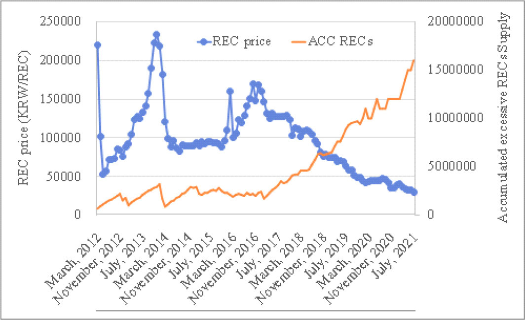
As shown in [Figure 1], the REC prices were highly unstable with periods of sharp increase and falls before 2017, but since the beginning of 2017, the REC spot market price has been falling continuously. Specifically, the REC prices dropped dramatically from about KRW 160,000 (USD 131) in the beginning of 2017 to less than KRW 30,000 (USD 25) in July 2021. There might be several reasons for such drop in the REC price. First, fast growth of solar PV (photovoltaic) in Korean energy market exceeded the RPS quota for the last several years, as a result, accumulated excessive REC supply increased considerably (from about 2 millions in 2017 to over 16 millions in July, 2021), so the REC price decreased dramatically. Second reason might be related with policy change in the REC market. Before 2017, power producers and renewable energy providers negotiated freely and forged long-term (12-year) contracts. In 2017, the government revised the auction system to integrate System Marginal Price (SMP) and REC price into a single fixed contract price (SMP + REC) and offered long term contracts for 20 years. So if renewable energy producers and mandatory power plants prefer to enter into the REC contract market, rather than trading on the spot market, in order to avoid the uncertainty of REC prices in the spot market, this policy change can have negative impact on REC prices. In order to account a potential effect of (SMP+REC) integrated contract price on the REC spot market price, we includes a dummy variable (Contract) which value is zero before 2017, and 1 otherwise. As mentioned in the introduction, the REC weight has been revised every 3 years. Therefore, we include an additional variable which is a maximum REC weight (Weight_Max) related to the highest REC weight in every given month to assess the effect of REC weights on the REC spot market prices. For example, the highest REC weight was applied to wind power (2.0) in 2012, while the ESS linked to solar and wind power plants had the highest weight (5.5) in 2016, so the value of Weight_Max variable will be 2.0 in 2012 and 5.5 in 2016, for example.
<Table 1>
Descriptive statistics
Ⅳ. Estimation models
Autoregressive Distributed Lag (ARDL) model is employed to investigate determinants of REC price. STATA with version17 was used to estimate ARDL model with the optimal number of autoregressive and distributed lags based on the Akaike or Schwarz/Bayesian information criterion. In the case of cointegration between variables, the ARDL model can be conveniently reparametrized in so-called error-correction (EC) form, which separates the long-run relationship from the short-run dynamics. One of the main advantages of the ARDL approach in cointegration analysis is that it can deal with a mixture of stationary and non-stationary variables with the first order of integration (Pesaran and Shin, 1999).
Basically, the ARDL model has the following form:
where the ARDL model of is explained by 2 components: the autoregressive component includes its own p lagged variables, and the lagged distribution of the other explanatory variables () with lags . is an intercept, and are lag orders, and and are parameters. The variables in and are allowed to be stationary I(0), integrated in order one I(1). In addition, if there is cointegration relationship between variables, it is necessary to apply the ARDL model in the EC representation (Hassler and Wolters, 2006).
where coefficients in equation (6) are mapped in a straightforward algebraic way to the coefficients in equation (5) are:
Expressions in the parentheses of equation (6) represent the deviation from the equilibrium or so-called error correction term (). An important role here plays the speed-of-adjustment coefficient α, which is the coefficient of the EC term . It tells us how fast the process for reverts back to its long-run relationship when the equilibrium is distorted. For existence of long-run relationship, this coefficient should satisfy . When 𝛼=0, then is I(1) and there is no long-run relationship. For a long-run level relationship to exist, we need both and . In order to determine whether variables in consideration have long-run relationship (Pesaran et al., 2001), bounds test was performed. In the first step, the F-statistic was used for testing the joint null hypothesis 𝛼=0 and . In the second step, the individual null hypothesis 𝛼=0 was tested by using the t-statistics from the Bound test. If the estimated values of the test statistics below the lower bound, null hypothesis of no long-run relationship cannot be rejected, but we can reject the null hypothesis if the test statistics exceeds the upper-bound critical value, and test results are inconclusive if test statistics fall between lower- and upper-bounds.
Before applying the ARDL model, the various unit root tests were applied to check the stability of time series data. Although ARDL model can deal with variables with mixed order of integration, it cannot be applied to variables with order of integration higher than one.
The specific ECM with the ARDL used to estimate the REC price is shown in equation (8).
where 𝛼 is the speed of adjustment parameter with a negative sign; are the long-run parameters; are short-run dynamic coefficients of the adjusted long-run equilibrium model; are coefficient of corresponding exogenous policy-related variables.
As a result of testing the relationship between stability and cointegration of time series, ARDL ECM was found to be suitable for this study. Moreover, ARDL ECM is more effective when the size of the data is small (Our data has 113 observations). In addition, this model allows the ordinary least squares (OLS) method to estimate the cointegration when the model lag is determined. This makes the ARDL ECM the best model in this case.
In addition to ARDL estimation, we estimate out-of-sample REC prices from August 2021 to July 2022.4) Forecast procedure is based on in-sample values of PREC_S (in periods T, T-1, ... 1) and estimated coefficients obtained from ARDL estimates for forecasting the future values of PREC_S (in periods T+1, T+2, ...). For this task, we can either hold our variables fixed at their last in-sample values or use actual (known) values (if available) for forecasted periods.
Ⅴ. Estimation Results
The Augmented Dickey-Fuller (ADF) and Phillips-Perron (PP) unit root tests were used to determine the stationarity of the time series. If the absolute value of the test statistics is greater than the absolute value of the critical value, we should reject H0 which means the series is stationary.
<Table 2> shows the details of the test results. Both tests indicate that the logarithm of PREC_S, ACCREC, and SMP are non-stationary in levels, but stationary in the first difference, which implies that these variables are integrated with order one (I(1)). On the other hand, the results suggest that the QREC_S is stationary in levels. Since all variables are integrated at most at order 1, it is possible to proceed with the estimation of the ARDL model. However, it should be noted that the presence of variables with a mixed order of integration makes it impossible to apply most cointegration approaches such as Johansen (1991) or Phillips and Hansen (1990). Nevertheless, the bound test for long-run relationship (Pesaran et al., 2001) can still be employed.
<Table 2>
Dickey-Fuller and Phillips-Perron unit root tests results
| Variable | order | ADF | PP | |
| t-statistics | t-statistics | Rho-statistics | ||
| InPREC_S | Level | -1.402 | -6.975 | -1.784 |
| 1st difference | -9.256*** | -70.189*** | -9.481*** | |
| InQREC_S | Level | -5.689*** | -21.982*** | -5.787*** |
| 1st difference | -15.097*** | -117.042*** | -17.621*** | |
| InACCREC | Level | -1.227 | -2.662 | -1.262 |
| 1st difference | -9.549*** | -90.197*** | -9.519*** | |
| InSMP | Level | -2.251 | -2.133 | -6.261 |
| 1st difference | -6.113*** | -10.925*** | -121.88*** | |
<Table 3> presents the results of the ARDL bound test for long-run relationship. The estimated value of F-statistics (8.493) is above the upper-bound even for 1% significant level (5.805), indicating the rejection of the null hypothesis of no level relationship. The absolute value of the t-statistics (3.707) is above the upper-bound critical value at 10% significance level, but within the bounds for the 5% and 1% significance levels. Overall, the statistical evidence is mixed, but there is mild support for the existence of a long-run level relationship at 10% significance level. Therefore, an estimation of EC representation of the ARDL is more appropriate.
<Table 4> shows the estimation results of the long-run coefficients in the ARDL_EC model. The Akaike information criterion (AIC) is used to select the optimum lag order (which selects the model that corresponds to its minimum value). According to the AIC, the ARDL (1, 0, 3, 0) model was selected as the preferred model, representing one lag for PREC_S, zero lags for QREC_S and SMP, and three lags for ACCREC. According to the study by Kripfganz and Schneider (2018), the EC representation can be formulated equivalently with the levels of the long-run forcing variables expressed in period instead of -1 when lag structure for some or all of the long-run forcing variables have zero lags (such as volume of RECs sold and SMP in our model). The interpretation of the long-run coefficients 𝜃 does not change in this case because the time subscript is irrelevant when the process is in equilibrium.
<Table 3>
Bound test results
As shown in <Table 4>, the estimated coefficient of the error correction (EC) term which is the speed of adjustment coefficient (α) has the expected negative sign and is statistically significant at 5% level, indicating the existence of a long run equilibrium. The value of the EC term suggests that a disturbance to the long-run equilibrium is corrected by 7% within one month to restore equilibrium in the dynamic model. The significance of the long-run coefficients is the final check for the existence of a level long-run relationship. The estimated long-run coefficient for QREC_S is positive and statistically significant at 5%, indicating that an increase in the QREC_S tends to increase PREC_S in the long run. Specifically, an increase in the QREC_S by 10% tends to increase PREC_S by 12.8%. The estimated long-run coefficient of ACCREC is highly significant (1% level) and has a negative sign, which is in line with economic theory. The estimated coefficient’s value shows that an increase in ACCREC by 10% would decrease PREC_S by 18.5%. The long-run coefficient for SMP is positive but statistically insignificant even at 10% level. This finding contradicts to Shrestha and Kakinaka (2023), who found that electricity prices (SMP) can have either a positive or negative impact on REC price. One reason for this discrepancy may be that this study considers long run effects and cannot examine time-varying effects. Another reason could be differences in electricity market policies in India and Korea, as the SMP in Korea is regulated by KPX public corporation based on supply and demand conditions in the market.
<Table 4>
Estimation of long-run coefficients in ARDL EC model
|
PREC_S (dependent variable) | QREC_S | ACCREC | SMP |
| Error correction term | -0.07**(0.029) | ||
| Long-run | 1.278**(0.538) | -1.853***(0.601) | 0.650 (0.704) |
<Table 5> shows the estimation of the short-run coefficients as well as estimated coefficients of exogeneous policy-related variables. As expected, increase in the ΔQREC_S leads to increase in the ΔPREC_S as short-run coefficient (for lag 0) is positive and statistically significant. Specifically, 10% increase in the ΔQREC_S results in increase of ΔPREC_S by 0.92%. The short-run coefficients of ΔACCREC are positive and statistically significant for lags t-1 and t-2 which indicate that higher fluctuations of ACCREC in previous periods tends to increase PREC_S fluctuation in period t. The estimated short-run coefficient of the SMP (ΔSMP) is positive, but statistically insignificant. Finally, the estimated coefficients of both REC policy-related variables are statistically significant with negative signs, which implies that higher REC weight and revision of long-term contract system had negative impacts on the REC spot market price.
<Table 5>
Estimation of short-run coefficients in ARDL EC model
|
∆PREC_S (dependent variable) | Lag 0 | Lag 1 | Lag 2 |
| ∆QREC_S | 0.092*** (0.017) | - | - |
| ∆ACCREC | 0.097 (0.065) | 0.134** (0.058) | 0.134** (0.058) |
| ∆SMP | 0.047 (0.048) | - | - |
| Constant | 1.616** (0.742) | ||
| Exogenous variables | |||
| WeightMax | -0.021** (0.010) | ||
| Contract | -0.069** (0.030) | ||
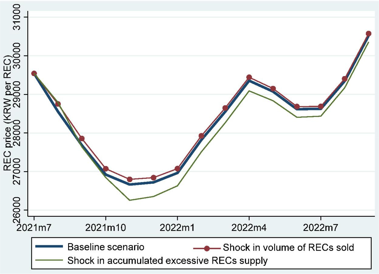
In addition to estimating the ARDL EC model, we predict the REC prices for next 14 months (based on data availability for SMP). We examined how shocks to the ACCREC and QREC_S would affect PREC_S. [Figure 2] shows the baseline and two alternative scenarios. The baseline scenario holds fixed values for ACCREC and QREC_S at their last in-sample values (July 2021), but used actual values for SMP, which are available up to July 2022. The alternative scenarios differ from the baseline scenario in the positive shock by magnitude 0.1 (10%) for the first out-of-sample month (August 2021) of ACCREC and QREC_S, respectively. As shown in [Figure 2], the baseline and alternative forecast scenarios reveal a decrease in PREC_S until November 2021, but then it starts to increase. This increase in PREC_S may be due to the MOTIE announcement in October 2021 about a change in the 2022 RPS target from 10% to 12.5% (by 2.5 percentage points). A shock in the QREC_S increases PREC_S compared to the baseline scenario, but this increase returns to the baseline scenario’s price within 12 months, as shown in [Figure 2]. However, a shock from the ACCREC increases PREC_S in the first period relative to the baseline scenario, but then the forecasted PREC_S goes below it.
Ⅵ. Summary and Policy Implication.
This study analyzed the determinants of REC spot market price by applying the ARDL estimation procedure. Specifically, we used the error correction model and examined the short-run and long-run relationships of the volume of RECs sold in the spot market, accumulated excessive REC supply, SMP, and related policy changes on REC spot market price. The estimation results showed that REC price can be affected by the volume of RECs sold in the spot market, accumulated excessive REC supply, but SMP was found to be statistically insignificant in the long run. Specifically, the volume of RECs sold in the spot market had a positive log run relationship with REC price, while accumulated excessive REC supply had a negative long-run relationship with the REC price.
The value of the EC term indicated that the disturbance from the long-run equilibrium was corrected by 7% within one month. Using the ARDL forecast procedure, we also showed that a 10% positive shock of the volume of RECs sold in the spot market reduces the REC price, relative to a 10% positive shock of accumulated excessive REC supply. Furthermore, it took longer for the REC price to return to the baseline scenario after a shock from the accumulated excessive REC supply, compared to a shock in the volume of RECs sold in the spot market. Similar to the prediction model, the short-run estimation results also revealed that higher fluctuations in accumulated excessive REC supply led to higher changes in REC prices. Moreover, inclusion of REC policy-related variables showed that the revision of the fixed price contract system reduced REC prices, probably because more REC buyers and sellers participated in the contract market to avoid uncertainties of REC prices in the spot market, as a result REC demand in the spot market fell and led to lower REC prices.
In fact, contract and spot REC markets are interconnected and together contribute to the overall efficiency of the REC market. Long-term contracts provide stability for project developers and support the growth of renewable energy capacity, while the spot market facilitates liquidity, price discovery, and flexibility in the trading of RECs. Together, they help facilitate the trading and exchange of RECs, ensuring compliance with RPS obligations and supporting the development of renewable energy projects. In addition, as expected, higher REC weights reduced REC prices, as higher weights implied more REC per 1 MWh, resulting in higher REC supply.
Based on the estimation results, we suggest the following policy implications for REC market stabilization. First, policy-makers can implement a policy to reduce the accumulation of RECs by applying a RECs depreciation system to avoid a significant increases of accumulated supply of the RECs. For example, if a mandatory power company received (by generating renewable electricity) or bought (in contract or spot market) the RECs but did not use them to fulfill the RPS target, it could be depreciated by 10% every 2 years (depreciation rate and periods are subject to change). Implementation of a such policy would lead to a gradual decrease in the value of purchased RECs by the mandatory power companies over the long term.
From the demand side, as our prediction model, as well as actual data, showed, in the third quarter of 2021, REC prices reached minimum but then started to increase, probably due to MOTIE’s announcement of an increased RPS target from 10% to 12.5% for 2022, and a gradual increase in the mandatory renewable energy ratio up to 25% by 2026. Such changes could lead to dramatic rises in demand for RECs, resulting in increased REC prices in the long-run. On the other hand, high REC prices may result in a higher accumulation of RECs due to the excessive entrance of renewable energy producers or installation of renewable energy facilities by mandatory power companies. In addition, a low REC price does not increase REC demand without a change in RPS requirements, as a result, the accumulation of RECs would increase without a rise in equilibrium price.
In summary, a smart management of the REC demand and supply will be required for efficient operation of the REC market. Otherwise, REC prices would continue to fluctuate significantly that would have a negative impact on attractiveness of investment in renewable energy sectors.
